ABSTRACT (original article): A Grossman-Stiglitz type model is proposed to solve two variance premium/VIX puzzles: Why do investors pay to hold realized variance risk, instead of earn a premium? And, why do they pay more in post-crisis months? The model consists of three periods. Agents are identical initially, then become heterogenous due to nontraded risk shocks and trade to hedge, and finally consume payoffs. The equilibrium provides a novel perspective on the time series of VIX, S&P500 returns, and SPY trading. The long time series, 1993 through 2024, includes several crises. These crises share a common pattern, which the model can generate endogenously. CITATION (original article): Menkveld, Albert J., Pricing Variance in a Model with Fire Sales (February 10, 2025). Available at SSRN: http://dx.doi.org/10.2139/ssrn.5043741
The structure of the notebook is as follows. It first develops the expressions for the liquidity demander in the model and then does the same for the liquidity supplier in the model. These expressions are then used to value the variance swap. The two key factors in the formula for the variance swap are the inflator for the flow-correlated return and the inflator for the flow-uncorrelated return. These expressions appear in Proposition 1 of the manuscript. The proof is in the Appendix of the manuscript.
Introduction
Introduction

The VIX is often referred to as the fear gauge. But, what exactly do investors fear?
My conjecture is that it is the fear of forced selling. I propose a Grossman-Stiglitz type model to show that, indeed, VIX could be a gauge of fire sales.
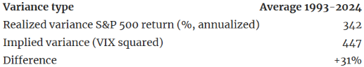
The Volatility Index (VIX) was launched in 1993 by the Chicago Board Options Exchange (CBOE). The CBOE refers to it as an “index to measure the market’s expectation of future volatility.”1 This is, at best, only partially true. If one compares the realized variance of S&P500 index returns to the variance implied by the VIX over the lifetime of the VIX, then the latter is 31% higher.
The structure of the notebook is as follows. It first develops the expressions for the liquidity demander in the model and then does the same for the liquidity supplier in the model. These expressions are then used to value the variance swap. The two key factors in the formula for the variance swap are the inflator for the flow-correlated return and the inflator for the flow-uncorrelated return. These expressions appear in Proposition 1 of the manuscript. The proof is in the Appendix of the manuscript.
Empirical patterns
Empirical patterns
This wedge between implied and realized variance is well known in the academic literature. It is referred to as the variance risk premium (VRP). It has been documented to be positive on average. And, it is significantly higher in the months after a crisis.
A positive VRP has been explained with time-varying volatility,2 but a rational explanation for an elevated VRP in the months after a crisis remains elusive.3
I have long had the intuition that the key to understand these puzzling findings might lie in trading the index. I analyzed SPY, which is arguably the largest exchange traded fund (ETF) that tracks the S&P 500 index. It was launched in 1993 and, therefore, intraday trade data is available since the inception of VIX in 1993. Simple averaging across crisis periods show that:
◼
SPY volume is 86% higher in post-crisis months.
◼
SPY liquidity is 18% worse, as judged by the bid-ask spread (depth declines even further).
Model
Model
The model expands the Grossman-Stiglitz type model proposed by Vayanos and Wang (2012, RFS). Information is symmetric across agents in their baseline version. I add a variance swap to this version of the model in order to price its payoff, i.e., being paid realized variance. The late Peter Carr eloquently argued that the price of such swap is approximately equal to VIX squared. Solving the model, therefore, yields an equilibrium expression for VIX. In closed form.
The model consists of three periods. Agents are identical initially, then become heterogeneous due to nontraded risk shocks which trigger trade, and, finally, they consume their payoffs. The engine of all results is the second period, in which the agents who experience the shock, become liquidity demanders to hedge the shock. The correlation of the shock is such that demanders need to sell in bear markets and buy in bull markets. This pattern could be interpreted as leverage-induced trading.
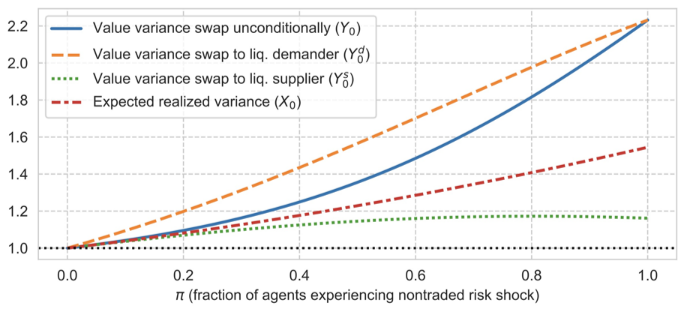
The figure above is the signature graph of the paper. It shows how the value of the variance swap, i.e., VIX squared, depends on the fraction of agents who experience the shock in period two. The blue solid line shows that this value monotonically increases in the fraction of shocked agents. It is a probability weighted sum of the value attached to the swap by shocked agents who become liquidity demanders, and the others who endogenously become liquidity suppliers. Demanders value the swap higher than expected realized variance. Suppliers value it lower.
Note that this expected realized variance itself increases in the fraction of shocked agents. This is due to (transitory) price pressures that are needed to clear the market. They compensate liquidity suppliers for taking on more risk. These pressures add to realized variance and, therefore, to the payoff of the variance swap.
Importantly, the model findings can explain the empirical patterns:
◼
The variance risk premium is proven to be nonnegative in the model.
◼
The model can explain the post-crisis pattern of elevated VRP, elevated volume, and worse liquidity.
An extremely short summary of the rich set of results that the model yields is: VIX is an index to measure (investor) utility cost of fire sales. One might say that the model puts flesh and bones on the popular saying that VIX is …
… a fear gauge.
Liquidity demander
Liquidity demander
This part derives how the liquidity demander values the swap in Period 1. In the manuscript, the notation for this valuation is y subscript 1, superscript d. This, however, cannot be done in Mathematica notebooks and, therefore, the notation used below is y1d. The same holds for other objects.
In[]:=
B1:=Simplify[{{σv2/σz+α*σv3^2*β},{0}}.{{σv2/σz+α*σv3^2*β,0}}+{{α*σv3^2*β},{1}}.{{α*σv3^2*β,1}}]B1//MatrixForm
Out[]//MatrixForm=
2 α 2 β 4 σv3 2 αβ 2 σv3 σv2 σz | αβ 2 σv3 |
αβ 2 σv3 | 1 |
B4d is B4 for demander as opposed to supplier.
B4d:=Simplify[(1/2)*{{1-β},{0}}.{{-α*σv3^2*β,0}}+Transpose[(1/2)*{{1-β},{0}}.{{-α*σv3^2*β,0}}]+(1/2)*{{-(1-β)+1},{0}}.{{0,1}}+Transpose[(1/2)*{{-(1-β)+1},{0}}.{{0,1}}]]B4d//MatrixForm
Out[]//MatrixForm=
α(-1+β)β 2 σv3 | β 2 |
β 2 | 0 |
In[]:=
Σ:={{σz^2,0},{0,σv3^2}}Σ//MatrixForm
Out[]//MatrixForm=
2 σz | 0 |
0 | 2 σv3 |
Intermediate step.
Inverse[Σ]+2*α*B4d//MatrixForm
Out[]//MatrixForm=
2 2 α 2 σv3 1 2 σz | αβ |
αβ | 1 2 σv3 |
Σs is SuperStar[Σ] in the manuscript.
Σsd:=FullSimplify[Inverse[Inverse[Σ]+2*α*B4d]]Σsd//MatrixForm
Out[]//MatrixForm=
2 σz 1+ 2 α 2 σv3 2 σz | - αβ 2 σv3 2 σz 1+ 2 α 2 σv3 2 σz |
- αβ 2 σv3 2 σz 1+ 2 α 2 σv3 2 σz | 2 σv3 2 α 4 σv3 2 σz 1+ 2 α 2 σv3 2 σz |
In[]:=
DetΣsd:=FullSimplify[Det[Σsd]]DetΣsd//MatrixForm
Out[]//MatrixForm=
2
σv3
2
σz
1+(-2+β)β
2
α
2
σv3
2
σz
In[]:=
DetΣ:=Det[Σ]DetΣ//MatrixForm
Out[]//MatrixForm=
2
σv3
2
σz
In[]:=
TrB1Σsd=FullSimplify[Tr[B1.Σsd]]
Out[]=
2
σv2
2
σv3
2
σv3
2
α
4
σv3
2
σz
1+(-2+β)β
2
α
2
σv3
2
σz
In[]:=
y1d:=FullSimplify[(DetΣsd/DetΣ)*TrB1Σsd]y1d//MatrixForm
Out[]//MatrixForm=
2
σv2
2
σv3
2
σv3
2
α
4
σv3
2
σz
2
(1+(-2+β)β)
2
α
2
σv3
2
σz
Above is the expression that Mathematica gives. Is it the same as the one in the manuscript? To check, below is the expression in the manuscript denoted by y1dAlt. To compare if they the same, the differential is evaluated. This differential should be a function that is always 0, and it is.
In[]:=
A:=1/(1-(2-β)*β*(α^2)*(σv3^2)*(σz^2))A//MatrixForm
Out[]//MatrixForm=
1
1-(2-β)β
2
α
2
σv3
2
σz
In[]:=
y1dAlt:=(A^2)*((σv2+α*(σv3^2)*β*σz)^2)+A*(σv3^2)y1dAlt//MatrixForm
Out[]//MatrixForm=
2
(σv2+αβσz)
2
σv3
2
(1-(2-β)β)
2
α
2
σv3
2
σz
2
σv3
1-(2-β)β
2
α
2
σv3
2
σz
In[]:=
Together[y1d-y1dAlt]//MatrixForm
Out[]//MatrixForm=
0
Liquidity supplier
Liquidity supplier
This part does the same check as was done for the liquidity demander above, but this time for the liquidity supplier.
In[]:=
B4s:=Simplify[(1/2)*{{-β},{0}}.{{-α*σv3^2*β,0}}+Transpose[(1/2)*{{-β},{0}}.{{-α*σv3^2*β,0}}]+(1/2)*{{β},{0}}.{{0,1}}+Transpose[(1/2)*{{β},{0}}.{{0,1}}]]B4s//MatrixForm
Out[]//MatrixForm=
α 2 β 2 σv3 | β 2 |
β 2 | 0 |
Intermediate step.
Inverse[Σ]+2*α*B4s//MatrixForm
Out[]//MatrixForm=
2 2 α 2 β 2 σv3 1 2 σz | αβ |
αβ | 1 2 σv3 |
Σsis
*
Σ
Σss:=FullSimplify[Inverse[Inverse[Σ]+2*α*B4s]]Σss//MatrixForm
Out[]//MatrixForm=
2 σz 1+ 2 α 2 β 2 σv3 2 σz | - αβ 2 α 2 β 1 2 σv3 2 σz |
- αβ 2 α 2 β 1 2 σv3 2 σz | 2 σv3 1 1+ 2 α 2 β 2 σv3 2 σz |
In[]:=
DetΣss:=FullSimplify[Det[Σss]]DetΣss//MatrixForm
Out[]//MatrixForm=
2
σv3
2
σz
1+
2
α
2
β
2
σv3
2
σz
In[]:=
TrB1Σss=FullSimplify[Tr[B1.Σss]]
Out[]=
2+-+2αβσv2σz
2
σv3
2
σv2
2
σv3
2
σv3
1+
2
α
2
β
2
σv3
2
σz
In[]:=
y1s:=(DetΣss/DetΣ)*TrB1Σssy1s//MatrixForm
Out[]//MatrixForm=
2+-+2αβσv2σz
2
σv3
2
σv2
2
σv3
2
σv3
1+
2
α
2
β
2
σv3
2
σz
1+
2
α
2
β
2
σv3
2
σz
In[]:=
B:=1/(1+(β^2)*(α^2)*(σv3^2)*(σz^2))B//MatrixForm
Out[]//MatrixForm=
1
1+
2
α
2
β
2
σv3
2
σz
In[]:=
y1sAlt:=(B^2)*((σv2+α*(σv3^2)*β*σz)^2)+B*(σv3^2)y1sAlt//MatrixForm
Out[]//MatrixForm=
2
(σv2+αβσz)
2
σv3
2
(1+)
2
α
2
β
2
σv3
2
σz
2
σv3
1+
2
α
2
β
2
σv3
2
σz
In[]:=
Together[y1s-y1sAlt]//MatrixForm
Out[]//MatrixForm=
0
Value variance swap
Value variance swap
This part uses the valuations of the demander and the supplier, that have been derived above, to derive the valuation of the investor unconditionally. That is, in Period 1, the investor knows that he will become demander in Period 2 with probability beta, and supplier with probability one minus beta.
In[]:=
y1:=FullSimplify[β*y1d+(1-β)*y1s]y1//MatrixForm
Out[]//MatrixForm=
β(++2αβσv2σz+2(-1+β)β)
2
σv2
2
σv3
2
σv3
2
α
4
σv3
2
σz
2
(1+(-2+β)β)
2
α
2
σv3
2
σz
(-1+β)(++2αβσv2σz+2)
2
σv2
2
σv3
2
σv3
2
α
2
β
4
σv3
2
σz
2
(1+)
2
α
2
β
2
σv3
2
σz
Make sure the condition holds for which the expected utility is finite. See Section 3.1 in manuscript.
(3^2)*((400/10000)/12)*(3^2)<1
Out[]=
True
In[]:=
Plot[{{y1/(0.040/12)}/.{σz->3,σv2->(0.2*(0.040/12))^(0.5),σv3->(0.8*(0.040/12))^(0.5),α->3},{y1d/(0.040/12)}/.{σz->3,σv2->(0.2*(0.040/12))^(0.5),σv3->(0.8*(0.040/12))^(0.5),α->3},{y1s/(0.040/12)}/.{σz->3,σv2->(0.2*(0.040/12))^(0.5),σv3->(0.8*(0.040/12))^(0.5),α->3}},{β,0,1},PlotLegends->{"Unconditional","Liq demander","Liq supplier"}]
Out[]=
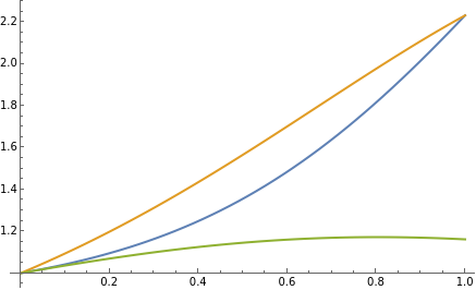
This plot mirrors the bottom plot of Figure 5 of the manuscript. The parameters are picked such that they are the same. The plot in the manuscript is produced by Python code. This is another check on the results reported in the manuscript.
Partial derivatives of inflators
Partial derivatives of inflators
This final part verifies the proof of Proposition 2 in the manuscript that the variance swap increases monotonically in β, α, and the variance of the endowment shock z. It does so by verifying that the partial derivative of the two inflators is strictly larger than zero in the permissible area.
The Reduce function in Mathematica allows one to “reduce” the area specified by a set of constraints. If the outcome (“image”) of Reduce function is the same as the area itself (“support”), then the constraints are not effectively reducing the area. For example, if Reduce(f(x)>0, x in A) gives back A, then f(x)>0 is true for all x in A. If it is only true for some subset of A, then the function Reduce would have given back a strictly smaller area than A.
The Reduce function in Mathematica allows one to “reduce” the area specified by a set of constraints. If the outcome (“image”) of Reduce function is the same as the area itself (“support”), then the constraints are not effectively reducing the area. For example, if Reduce(f(x)>0, x in A) gives back A, then f(x)>0 is true for all x in A. If it is only true for some subset of A, then the function Reduce would have given back a strictly smaller area than A.
Inflator flow-correlated return
Inflator flow-correlated return
In[]:=
InflCorrRet:=β*(A^2)+(1-β)*(B^2)
In[]:=
DInflCorrRetβ:=Simplify[D[InflCorrRet,β]](*Thiscomputesthepartialderivativeoftheinflatorofthecorrelatedreturnw.r.t.β.*)DInflCorrRetβ//MatrixForm
Out[]//MatrixForm=
-(4β(-1+3(-1+β)β+(10-18β+9)+(-8+18β-15+5)))()
2
α
2
σv3
2
σz
2
α
2
σv3
2
σz
4
α
2
β
2
β
4
σv3
4
σz
6
α
3
β
2
β
3
β
6
σv3
6
σz
3
(1+(-2+β)β)
2
α
2
σv3
2
σz
3
(1+)
2
α
2
β
2
σv3
2
σz
This part checks if, indeed, this partial derivative is strictly positive in the permissible area.
Reduce[(DInflCorrRetβ>0)&&(α>0)&&(σv3>0)&&(σz>0)&&(β>0)&&(β<1)&&((α^2)*(σv3^2)*(σz^2)<1),β]
Out[]=
σz>0&&σv3>0&&0<α<&&0<β<1
1
σv3σz
In[]:=
DInflCorrRetα:=Simplify[D[InflCorrRet,α]]DInflCorrRetα//MatrixForm
Out[]//MatrixForm=
4α+
2
β
2
σv3
2
σz
2-β
3
(1+(-2+β)β)
2
α
2
σv3
2
σz
-1+β
3
(1+)
2
α
2
β
2
σv3
2
σz
In[]:=
Reduce[(DInflCorrRetα>0)&&(α>0)&&(σv3>0)&&(σz>0)&&(β>0)&&(β<1)&&((α^2)*(σv3^2)*(σz^2)<1),α]
Out[]=
σz>0&&σv3>0&&0<β<1&&0<α<
1
σv3σz
In[]:=
DInflCorrRetσz:=Simplify[D[InflCorrRet,σz]]DInflCorrRetσz//MatrixForm
Out[]//MatrixForm=
4σz+
2
α
2
β
2
σv3
2-β
3
(1+(-2+β)β)
2
α
2
σv3
2
σz
-1+β
3
(1+)
2
α
2
β
2
σv3
2
σz
In[]:=
Reduce[(DInflCorrRetσz>0)&&(α>0)&&(σv3>0)&&(σz>0)&&(β>0)&&(β<1)&&((α^2)*(σv3^2)*(σz^2)<1),σz]
Out[]=
σv3>0&&0<β<1&&α>0&&0<σz<
1
ασv3
Inflator flow-non-correlated return
Inflator flow-non-correlated return
In[]:=
InflNoncorrRet:=β*A+(1-β)*B
In[]:=
DInflNoncorrRetβ:=D[InflNoncorrRet,β]DInflNoncorrRetβ//MatrixForm
Out[]//MatrixForm=
-+--
β(-(2-β)+β)
2
α
2
σv3
2
σz
2
α
2
σv3
2
σz
2
(1-(2-β)β)
2
α
2
σv3
2
σz
1
1-(2-β)β
2
α
2
σv3
2
σz
2(1-β)β
2
α
2
σv3
2
σz
2
(1+)
2
α
2
β
2
σv3
2
σz
1
1+
2
α
2
β
2
σv3
2
σz
In[]:=
Simplify[-β(-((2-β))+β)]
2
α
2
σv3
2
σz
2
α
2
σv3
2
σz
Out[]=
-2(-1+β)β
2
α
2
σv3
2
σz
In[]:=
Reduce[(DInflNoncorrRetβ>0)&&(α>0)&&(σv3>0)&&(σz>0)&&(β>0)&&(β<1)&&((α^2)*(σv3^2)*(σz^2)<1),β]
Out[]=
σz>0&&σv3>0&&0<α<&&0<β<1
1
σv3σz
In[]:=
DInflNoncorrRetα:=Simplify[D[InflNoncorrRet,α]]DInflNoncorrRetα//MatrixForm
Out[]//MatrixForm=
2α+
2
β
2
σv3
2
σz
2-β
2
(1+(-2+β)β)
2
α
2
σv3
2
σz
-1+β
2
(1+)
2
α
2
β
2
σv3
2
σz
In[]:=
Reduce[(DInflNoncorrRetα>0)&&(α>0)&&(σv3>0)&&(σz>0)&&(β>0)&&(β<1)&&((α^2)*(σv3^2)*(σz^2)<1),α]
Out[]=
σz>0&&σv3>0&&0<β<1&&0<α<
1
σv3σz
In[]:=
DInflNoncorrRetσz:=Simplify[D[InflNoncorrRet,σz]]DInflNoncorrRetσz//MatrixForm
Out[]//MatrixForm=
2σz+
2
α
2
β
2
σv3
2-β
2
(1+(-2+β)β)
2
α
2
σv3
2
σz
-1+β
2
(1+)
2
α
2
β
2
σv3
2
σz
In[]:=
Reduce[(DInflNoncorrRetσz>0)&&(α>0)&&(σv3>0)&&(σz>0)&&(β>0)&&(β<1)&&((α^2)*(σv3^2)*(σz^2)<1),σz]
Out[]=
σv3>0&&0<β<1&&α>0&&0<σz<
1
ασv3
In[]:=
Plot[{{InflCorrRet}/.{σz->3,σv2->(0.2*(0.040/12))^(0.5),σv3->(0.8*(0.040/12))^(0.5),α->3},{InflNoncorrRet}/.{σz->3,σv2->(0.2*(0.040/12))^(0.5),σv3->(0.8*(0.040/12))^(0.5),α->3}},{β,0,1},PlotLegends->{"InflCorrRet","InflNoncorrRet"}]
Out[]=
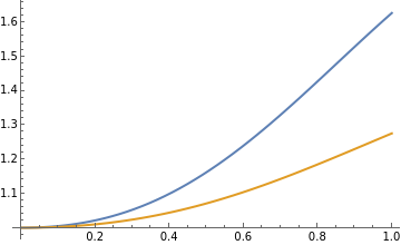
This plot mirrors the top plot of Figure 5 of the manuscript. The parameters are picked such that they are the same. The plot in the manuscript is produced by Python code. This is another check on the results reported in the manuscript.
CITE THIS NOTEBOOK
CITE THIS NOTEBOOK
Pricing variance in a model with fire sales
by Albert J. Menkveld
Wolfram Community, STAFF PICKS, February 20, 2025
https://community.wolfram.com/groups/-/m/t/3398135
by Albert J. Menkveld
Wolfram Community, STAFF PICKS, February 20, 2025
https://community.wolfram.com/groups/-/m/t/3398135