Abstract
Abstract
In Example 1 the Wolfram Language was used to give sets of flat curves volume. The experimental transition from 2D to 3D was animated. Example 2 visualized forming compounds of polyhedra and revealing their hidden “core”.
Experiment
Experiment
Example 1: Depth
Example 1: Depth
Variant 1:
Variant 1:
In[]:=
path0=SetDirectory[NotebookDirectory[]<>"/data/"]
Out[]=
D:\DDocs\0-published\woco\ams12pub\data
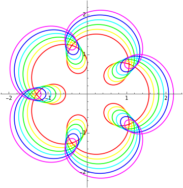
The set of curves was plotted in 2D:
In[]:=
CurveSetPlot2D[f_]:=Block[{a,funs,t},a=Table[i/16,{i,1,11,2}];funs=Table[f+a[[i]]*{Cos[t],Sin[t]},{i,1,6}];Show[Table[ParametricPlot[funs[[i]],{t,0,2Pi},PlotStyle->Hue[(i-1)/6],PlotRange->All],{i,1,6}]]]
In[]:=
f={Cos[t]+Cos[6t]/2,Sin[t]+Sin[6t]/2};CurveSetPlot2D[f]
Out[]=
The first and second coordinate of each curve from above were combined to form the third coordinate via the anonymous function (3-Norm[#]^2)&. With the function g (e.g. (E^#/4)&, (Sqrt[#]/2)&) applied to (3-Norm[#]^2)& the shape of the resulting 3D-graphics could be varied further in an experimental way.
In[]:=
CurveSetPlot3D[f_,g_]:=Block{a,funs,funs2,t,z},a=,,,,,;funs=(f+#*{Cos[t],Sin[t]})&/@a;funs2=({#[[1]],#[[2]],g[(3-Norm[#]^2)]})&/@funs;Show[ParametricPlot3D[#,{t,0,2Pi},ColorFunction"Rainbow",PlotRange->All,Boxed->False,Axes->False]&/@funs2]
1
16
3
16
5
16
7
16
9
16
11
16
In[]:=
f={Cos[t]+Cos[6t]/2,Sin[t]+Sin[6t]/2};
The divisor in g was adapted for scaling:
In[]:=
g=(#)&;pp3=CurveSetPlot3D[f,g]
Out[]=

In[]:=
g=(#/2)&;pp3=CurveSetPlot3D[f,g]
Out[]=

In[]:=
g=(E^(-#)/4)&;pp3=CurveSetPlot3D[f,g]
Out[]=

In[]:=
f={Cos[t]+Cos[5t]/2,Sin[t]+Sin[5t]/2};
In[]:=
g=(E^#/4)&;pp3=CurveSetPlot3D[f,g]
Out[]=

In[]:=
f={Cos[t]+Cos[8t]/2,Sin[t]+Sin[8t]/2};
In[]:=
g=(Sqrt[#]/2)&;pp3=CurveSetPlot3D[f,g]
Out[]=

In[]:=
g=(Tan[#/9])&;pp3=CurveSetPlot3D[f,g]
Out[]=

Variant 2:
Variant 2:
For the second set of curves an additional function h was introduced:
In[]:=
path0=SetDirectory[NotebookDirectory[]<>"/data/"]
Out[]=
D:\DDocs\0-published\woco\ams13pub\data
CurveSetPlot2DV2[f_,h_]:=Block[{a,funs,t},a=Table[i/16,{i,1,11,2}];funs=Table[f{Cos[t],Sin[t]}+a[[i]]{Cos[h],Sin[h]},{i,1,6}];Show[Table[ParametricPlot[funs[[i]],{t,0,2Pi},PlotStyle->Hue[(i-1)/6],PlotRange->All],{i,1,6}]]]
f=Sin[3t]+1;h=t+Pi/9*f;CurveSetPlot2DV2[f,h]
∂
t
In[]:=
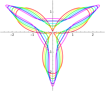
In[]:=
CurveSetPlot3DV2[f_,h_,g_]:=Block{a,funs,funs2,t,z},a=,,,,,;funs=(f*{Cos[t],Sin[t]}+#{Cos[h],Sin[h]})&/@a;funs2=({#[[1]],#[[2]],g[(3-Norm[#]^2)]})&/@funs;Show[ParametricPlot3D[#,{t,0,2Pi},ColorFunction"Rainbow",PlotRange->All,Boxed->False,Axes->False]&/@funs2]
1
16
3
16
5
16
7
16
9
16
11
16
In[]:=
f=Sin[6t]+1;h=t+Pi/9*f;
∂
t
In[]:=
g=(#/2)&;pp3=CurveSetPlot3DV2[f,h,g]
Out[]=

In[]:=
f=Sin[5t]+1;h=t+Pi/9*f;
∂
t
In[]:=
g=(E^(-#)/25)&;pp3=CurveSetPlot3DV2[f,h,g]
Out[]=

In[]:=
f=Sin[6t]+1;h=t+Pi/9*f;
∂
t
In[]:=
g=(E^(#)/4)&;pp3=CurveSetPlot3DV2[f,h,g]
Out[]=

In[]:=
f=Sin[5t]+1;h=t+Pi/9*f;
∂
t
In[]:=
g=(Sqrt[#]/4)&;pp3=CurveSetPlot3DV2[f,h,g]
Out[]=

In[]:=
f=Sin[8t]+1;h=t+Pi/9*f;
∂
t
In[]:=
g=(Tan[#/4])&;pp3=CurveSetPlot3DV2[f,h,g]
Out[]=

Five of the above 3D-graphics were exported as dxf-file, similar to:
In[]:=
Export["last.dxf",pp3]
Out[]=
last.dxf
Animation
Animation
Before animating the last example proper bounds had to be extracted:
In[]:=
rb=RegionBounds[DiscretizeGraphics[pp3]]
Out[]=
{{-2.64386,2.64402},{-2.64393,2.64397},{-1.76642,0.929774}}
The set of curves was scaled down incrementally by -0.1 in reference to the lowest z-value:
grTable=Graphics3D[GeometricTransformation[pp3[[1]],ScalingTransform[#,{0,0,1},{0,0,rb[[3,1]]}]],BoxedFalse,PlotRange->rb]&/@Reverse[Range[0.1,1,0.1]];
ListAnimate[grTable]
Out[]=

Blender
Blender
Part 1-5:
A dark metallic material was given to the ground plane. The curve sets were imported from dxf-files. The end-mapping of the curves was changed from 0 to 1 in a first animation. The second animation varied the z-scaling from 1 to 0.1 resulting in flattening the curve sets. Then the curve sets were grounded in a final animation by slowly decreasing the z-value of the curves below the z-value of the ground plane. A different material was chosen for each of the five curve sets. In the Video Editing Mode of Blender the sequence of the second and fourth curve set were reversed.
A dark metallic material was given to the ground plane. The curve sets were imported from dxf-files. The end-mapping of the curves was changed from 0 to 1 in a first animation. The second animation varied the z-scaling from 1 to 0.1 resulting in flattening the curve sets. Then the curve sets were grounded in a final animation by slowly decreasing the z-value of the curves below the z-value of the ground plane. A different material was chosen for each of the five curve sets. In the Video Editing Mode of Blender the sequence of the second and fourth curve set were reversed.
Example 2: Polyhedra
Example 2: Polyhedra
In[]:=
In[]:=
path0=SetDirectory[NotebookDirectory[]<>"/data/"]
Out[]=
D:\DDocs\0-published\woco\ams12pub\data
Animation of an Elevated Polyhedron
Animation of an Elevated Polyhedron
For the elevation on each face of the cube a pyramid with equilateral triangles as faces was added. The Wolfram Language code below recreated the first part of the animation Polyhedra:
In[]:=
gr1=Graphics3D[{Cuboid[{-0.5,-0.5,-0.5}],GeometricTransformation[Pyramid[{{-0.5,-0.5,#},{0.5,-0.5,#},{0.5,0.5,#},{-0.5,0.5,#},{0,0,0.5+1/Sqrt[3]}}],Table[RotationMatrix[iDegree,{1,0,0}],{i,0,270,90}]],GeometricTransformation[Pyramid[{{#,-0.5,-0.5},{#,0.5,-0.5},{#,0.5,0.5},{#,-0.5,0.5},{#+1/Sqrt[3],0,0}}],Table[RotationMatrix[iDegree,{0,0,1}],{i,0,180,180}]]},Boxed->False,Axes->False]&/@Table[i,{i,0.5,0.8,0.05}];ListAnimate[gr1]
Out[]=

Compounds of Polyhedra
Compounds of Polyhedra
A list of stellated polyhedra was extracted via Wolfram Alpha:
In[]:=

Out[]=
,,,,,,,,,,,,,,,,,
Three of the above list were selected:
In[]:=
chosen=,,;#["Graphics3D"]&/@chosen
Out[]=
 ,
, ,
,
For the Stella Octangula two tetrahedra were combined:
In[]:=
gr2=Graphics3D[{Tetrahedron[],Translate[GeometricTransformation[Tetrahedron[],RotationMatrix[180Degree,{0,1,0}]],{0,#,0}]},Boxed->False]&/@Table[i,{i,3,0,-0.5}];ListAnimate[gr2]
Out[]=

The “core” was created as intersection of the tetrahedra:
In[]:=
CSGRegion["Intersection",{Tetrahedron[],GeometricTransformation[Tetrahedron[],RotationMatrix[180Degree,{0,1,0}]]}]
Out[]=
Contents cannot be rendered at this time; please try again later or download this notebook for full functionality »
The stellation of the resulting octahedron lead back to the stellated octahedron.
For the cubo-octahedron compound a cube was combined with a resizable octahedron.
In[]:=
gr3=Graphics3D[{Cuboid[{-1,-1,-1},{1,1,1}],GeometricTransformation[Octahedron[],ScalingTransform[#{1,1,1}]]},Boxed->False]&/@Table[i,{i,2.5,2.8,0.05}];ListAnimate[gr3]
Out[]=

The “core” was created as intersection of the cube and octahedron:
In[]:=
CSGRegion["Intersection",{Cuboid[{-1,-1,-1},{1,1,1}],GeometricTransformation[Octahedron[],ScalingTransform[2.8{1,1,1}]]}]
Out[]=
Contents cannot be rendered at this time; please try again later or download this notebook for full functionality »
The augmentation of the resulting cuboctahedron lead back to the cubo-octahedron-compound.
As start for the Escher solid a combination of three rotated octahedra (45° around x, y, z-axis) was chosen.
In[]:=
directions={{1,0,0},{0,1,0},{0,0,1}};gr4=Graphics3D[Table[GeometricTransformation[Octahedron[],RotationMatrix[#Degree,directions[[i]]]],{i,1,3}],Boxed->False]&/@Table[i,{i,0,45,5}];ListAnimate[gr4]
Out[]=

The intersection of the octahedra formed the “core”:
In[]:=
CSGRegion["Intersection",Table[GeometricTransformation[Octahedron[],RotationMatrix[45Degree,directions[[i]]]],{i,1,3}]]
Out[]=
Contents cannot be rendered at this time; please try again later or download this notebook for full functionality »
Then one octahedron of the compound was made smaller along the z-axis until the edges became parallel:
In[]:=
directions={{1,0,0},{0,1,0},{0,0,1}};gr5=Table[Graphics3D[GeometricTransformation[Octahedron[],RotationMatrix[45Degree,directions[[i]]]],Boxed->False],{i,1,3}];gr6=Show[Graphics3D[GeometricTransformation[gr5[[3,1]],ScalingTransform[0.7,{0,0,1},{0,0,0}]],Boxed->False],gr5[[1]],gr5[[2]]]
Out[]=

Blender
Blender
Part 1: Color Blue
Via Geometry Nodes a quadratic pyramid with equilateral faces was applied to all faces of the cube. The cube and the pyramid were given materials, developed procedurally. The opening from the compound polyhedron was animated. In the opened state a second rotational animation followed.
Part 2: Color Yellow
Two tetrahedra were brought together in an animation. The outer compound polyhedron nearly disappeared in the next animation (key-framing alpha channel) followed by a rotation of the “core” around the z-axis (with help of an empty object). Finally the outer hull was made opaque again.
Part 3: Color Red
A cube and an octahedron were translated to a meeting point. Again in an animation was played with visibility to showcase the “core” and its complement.
Part 4: Color Green
An animation showed the formation of a compound by three rotated octahedra. One of the octahedra was made smaller vertically until building parallel edges. The core was brought to attention again through rotation and by changing visibility.
References
References
Collection of animations
Collection of animations
References
Depth
Scene: Sets of 2D Curves modified to 3D
Arthur, Christopher. “Geometric Design, An Artful Portfolio of Mathematical Graphics.” Accessed May 23, 2022. https://wolfram.com/books/profile.cgi?id=9169.
“Wolfram Language & System Documentation Center,” May 23, 2022. https://reference.wolfram.com/language/.
Audio:
Stock Music & Sound Effects - Royalty Free Audio - Storyblocks
https://storyblocks.com/audio (accessed 2022-05-23)
MEDIA MUSIC GROUP. Evening In The Distance - Atmospheric Emotional Acoustic. Accessed May 23, 2022. SBA-346804151.
Polyhedra
Scene: Modified Elevated & Stellated Polyhedra
Sriraman, Bharath. Handbook of the Mathematics of the Arts and Sciences. Accessed May 29, 2022. https://link.springer.com/book/10.1007/978-3-319-57072-3.
“List of Stellated Polyhedra - Wolfram|Alpha.” Accessed May 29, 2022. https://wolframalpha.com.
Audio:
Stock Music & Sound Effects - Royalty Free Audio - Storyblocks
https://storyblocks.com/audio (accessed 2022-05-29)
William, Pearson. Tumbling Stars. Accessed May 29, 2022. Asset ID: SBA-300193126.