ABSTRACT (original article): The phenomenon of spontaneous emission can lead to the creation of an imaginary coupling and a shift. To explore this, we utilized the renormalized first Nikitin model, revealing an exponential detuning variation with a phase and an imaginary coupling along with the shift. By employing the time-dependent Schrödinger equation, we investigated the behavior of our system. Our findings indicate that the imaginary coupling provides specific information, while the shift generates allowed and forbidden zones in the energy diagram of the real part of the energy. In the diagram of the imaginary part of the energy, time dictates order or chaos in the system and identifies the information transmission zone. Notably, the first Nikitin model exhibits similarities to the Rabi model in the short-time approximation. Our theoretical conclusions are consistent with numerical solutions. CITATION (original article): A. D. Kammogne, L. C. Fai (2024), Spontaneous emission in an exponential model, arXiv:2412.07553. https://doi.org/10.48550/arXiv.2412.07553
The paper entitled ‘Spontaneous emission in an exponential model’ discusses spontaneous emission through imaginary coupling and shifts caused by the interaction of particles with the magnetic field in an exponential model. This results in the formation of permitted or forbidden zones depending on the shift value, enabling control of quantum information. Using Mathematica software, we will see that the theoretical results align with the numerical results regarding the evolution of the ground state and excited state populations.
I. Real and imaginary part of energy
I. Real and imaginary part of energy
We define the constants, variables, and functions concerning this part
In[]:=
A:=1;(*Populationamplitude*)t:=7;(*time*)Alpha:=-15;(*sweeprate*)ϵ:=1;(*shift*)omega[β_]:=AExp[Alphat+β]+ϵ;(*detuning*)Delta[delta_]:=(delta+ϵ);(*Rabifrequency*)
In[]:=
theta[β_,delta_]:=ArcTan-;(*time-dependentangle*)
1
2
Delta[delta]
omega[β]
In[]:=
E1[β_,delta_]:=(Delta[delta]Csc[2theta[β,delta]]);(*Positiveenergy*)E2[β_,delta_]:=-(Delta[delta]Csc[2theta[β,delta]]);(*negativeenergy*)
In[]:=
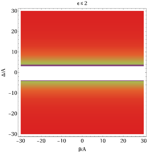
DensityPlot[{Re[E1[β,delta]]},{β,-30,30},{delta,-30,30},ColorFunction"Rainbow",PlotLegendsBarLegend[Automatic,LegendMarkerSize500,LegendMargins5,LegendLabel"Re()"],ImageSize500,FrameTrue,AxesNone,LabelStyle{FontFamily"Times New Roman",19,GrayLevel[0]},FrameStyle{{Black,Black},{Black,Black}},FrameLabel{"β/A","Δ/A","ϵ ≤ 2"}]
E
+
Out[]=

In[]:=
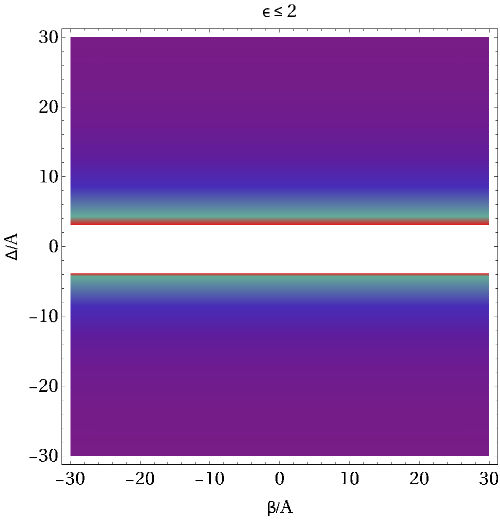
DensityPlot[{Re[E2[β,delta]]},{β,-30,30},{delta,-30,30},ColorFunction"Rainbow",PlotLegendsBarLegend[Automatic,LegendMarkerSize500,LegendMargins5,LegendLabel"Re()"],ImageSize500,FrameTrue,AxesNone,LabelStyle{FontFamily"Times New Roman",19,GrayLevel[0]},FrameStyle{{Black,Black},{Black,Black}},FrameLabel{"β/A","Δ/A","ϵ ≤ 2"}]
E
-
Out[]=
In[]:=
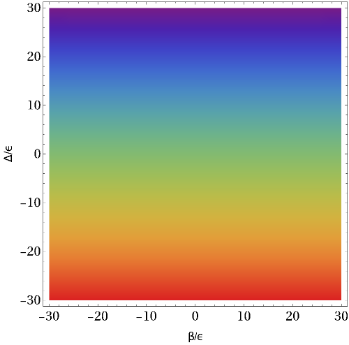
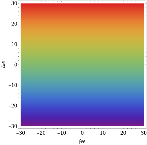
DensityPlot[{Im[E1[β,delta]]},{β,-30,30},{delta,-30,30},ColorFunction"Rainbow",PlotLegendsBarLegend[Automatic,LegendMarkerSize500,LegendMargins5,LegendLabel"Im ()"],ImageSize500,FrameTrue,AxesNone,LabelStyle{FontFamily"Times New Roman",19,GrayLevel[0]},FrameStyle{{Black,Black},{Black,Black}},FrameLabel{"β/ϵ","Δ/ϵ"}]
E
+
Out[]=

In[]:=
DensityPlot[{Im[E2[β,delta]]},{β,-30,30},{delta,-30,30},ColorFunction"Rainbow",PlotLegendsBarLegend[Automatic,LegendMarkerSize500,LegendMargins5,LegendLabel"Im ()"],ImageSize500,FrameTrue,AxesNone,LabelStyle{FontFamily"Times New Roman",19,GrayLevel[0]},FrameStyle{{Black,Black},{Black,Black}},FrameLabel{"β/ϵ","Δ/ϵ"}]
E
-
Out[]=
In[]:=
Clear[A,ϵ,t](*it'simportanttoclearthepreviousvaluesofsomeparameters*)
II. Survival and transitions probabilities
II. Survival and transitions probabilities
In this notebook, we only treat the case where the populations of the ground and excited states vary as a function of time, while other cases concerning coupling and shift can be conjectured using certain constants as parameters .
We define the constants, variables, and functions concerning this part
In[]:=
t0:=0.0;A:=2.0;ϵ:=2.0;α:=1.0;β:=1.5;Δ:=0.0;
In[]:=
a:=1-;b:=;c:=;
ϵ
α
A
α
Δ+ϵ
2α
In[]:=
μ:=1-a+-4;γ:=1+-4;λ:=;z[t_]:=Exp[αt+β];
1
2
2
(1-a)
2
c
2
(1-a)
2
c
ϵ
2α
In[]:=
G[t1_,t2_]:=Hypergeometric1F1[μ,γ,bz[t1]]HypergeometricU[μ,γ,bz[t2]];ϑ[t1_,t2_]:=(λ+μ)Log[z[t1]]+(γ-1-μ-λ)Log[z[t2]]-(z[t1]+z[t2]);U12[t1_,t2_]:=c(G[t1,t2]-G[t2,t1])Exp[ϑ[t1,t2]];Probability1[t_]:=Re[U12[t,t0]]^2+Im[U12[t,t0]]^2;
b
2
γ-1
b
Gamma[μ]
Gamma[γ]
In[]:=
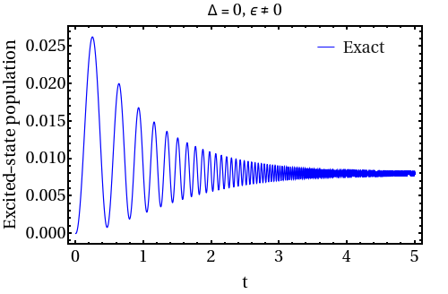
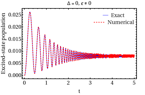
Np=Plot[Probability1[t],{t,0,5},PlotRangeAll,PlotStyle{Thickness[0.003],Blue},ImageSize500,FrameTrue,AxesNone,PlotLegendsPlaced[{"Exact"},{0.8,0.9}],LabelStyle{FontFamily"Times New Roman",19,GrayLevel[0.1]},FrameStyleDirective[Thick,19,Black],FrameLabel{"t","Excited-state population","Δ = 0, ϵ ≠ 0",""}]
Out[]=
In[]:=
t0:=0;tfin:=5;sol1=NDSolvey1'[t]-((A*Exp[αt+β]+ϵ)y1[t]+(Δ+ϵ)y2[t])0,y2'[t]-((-A*Exp[αt+β]-ϵ)y2[t]+(Δ+ϵ)y1[t])0,y1[t0]0,y2[t0]1,{y1,y2},{t,t0,tfin}
1
2
1
2
Out[]=
y1InterpolatingFunction,y2InterpolatingFunction
In[]:=
Prob1[t_]:=Re[Evaluate[y1[t]/.sol1]]^2+Im[Evaluate[y1[t]/.sol1]]^2;Prob2[t_]:=Re[Evaluate[y2[t]/.sol1]]^2+Im[Evaluate[y2[t]/.sol1]]^2;
In[]:=
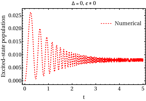
Mp=Plot[Prob1[t],{t,0,5},PlotRangeAll,PlotStyle{Thickness[0.006],Dashed,Thickness[0.006],{Blue,Red}},PlotLegendsPlaced[{"Numerical"},{0.8,0.8}],ImageSize500,FrameTrue,AxesNone,LabelStyle{FontFamily"Times New Roman",19,GrayLevel[0.1]},FrameStyleDirective[Thick,19,Black],FrameLabel{"t","Excited-state population","Δ = 0, ϵ ≠ 0"}]
Out[]=
In[]:=
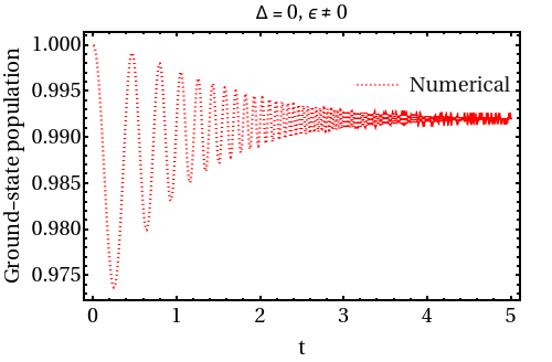
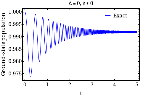
Mp1=Plot[Prob2[t],{t,0,5},PlotRangeAll,PlotStyle{Thickness[0.006],Dashing[Tiny],Thickness[0.006],{Blue,Red}},PlotLegendsPlaced[{"Numerical"},{0.8,0.8}],ImageSize500,FrameTrue,AxesNone,LabelStyle{FontFamily"Times New Roman",19,GrayLevel[0.1]},FrameStyleDirective[Thick,19,Black],FrameLabel{"t","Ground-state population","Δ = 0, ϵ ≠ 0",""}]
Out[]=
In[]:=
U22[t1_,t2_]:=μG[t1,t2]-G[t2,t1]+Hypergeometric1F1[μ+1,γ+1,bz[t1]]HypergeometricU[μ,γ,bz[t2]]+bz[t1]Hypergeometric1F1[μ,γ,bz[t2]]HypergeometricU[μ+1,γ+1,bz[t1]]Exp[ϑ[t1,t2]];Probability2[t_]:=Re[U22[t,t0]]^2+Im[U22[t,t0]]^2;
γ-1
b
Gamma[μ]
Gamma[γ]
bz[t1]
γ
In[]:=
Np1=Plot[Probability2[t],{t,0,5},PlotRangeAll,PlotStyle{Thickness[0.003],Blue},ImageSize500,FrameTrue,AxesNone,PlotLegendsPlaced[{"Exact"},{0.8,0.9}],LabelStyle{FontFamily"Times New Roman",19,GrayLevel[0.1]},FrameStyleDirective[Thick,19,Black],FrameLabel{"t","Ground-state population","Δ = 0, ϵ ≠ 0",""}]
Out[]=
In[]:=
Show[Np,Mp]
Out[]=
III. Similarity with rabi model
III. Similarity with rabi model
In[]:=
Clear[A](*it'simportanttoclearthepreviousvalueoftheamplitude*)
In[]:=
tin:=0;tfin:=5;A:=1;De:=0.2;ϑ[B_]:=ArcTan-;
1
2
(De+B)
B
In[]:=
u[t_,B_]:=-Exp-tSint;Probability2[t_,B_]:=Re[u[t,B]]^2+Im[u[t,B]]^2;
Csc[2ϑ[B]]
(B)
2
(De+B)Csc[2ϑ[B]]
2
In[]:=
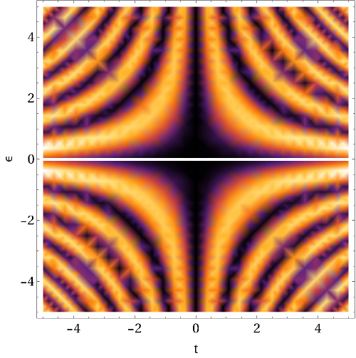
uq=DensityPlot[Probability2[t,B],{t,-5,5},{B,-5,5},ColorFunction"SunsetColors",PlotLegendsBarLegend[Automatic,LegendMargins1,LegendMarkerSize420,LegendLabel"(t)"],ImageSize500,FrameTrue,AxesNone,LabelStyle{FontFamily"Times New Roman",19,GrayLevel[0]},FrameStyle{{Black,Black},{Black,Black}},FrameLabel{"t","ϵ"}]
P
Rab1
Out[]=
CITE THIS NOTEBOOK
CITE THIS NOTEBOOK
Spontaneous emission in an exponential model
by Kammogne Djoum Nana Anicet & L. C. Fai
Wolfram Community, STAFF PICKS, July 7, 2025
https://community.wolfram.com/groups/-/m/t/3493438
by Kammogne Djoum Nana Anicet & L. C. Fai
Wolfram Community, STAFF PICKS, July 7, 2025
https://community.wolfram.com/groups/-/m/t/3493438