Identification of homogeneity in Wolfram Model hypergraphs via approximate Isomorphism
by Regen Petu-Stiles, Imperial College London
[WWS22]
by Regen Petu-Stiles, Imperial College London
[WWS22]
This project aimed to identify Statistical Uniformity in Hypergraphs as a means to highlight analogues to the Classical Vacuum within the Wolfram Model. First, one must create a rule set that can be considered a discrete approximation to a spacelike hypersurface to model a candidate “universe”. To analyse the resulting structures, one will be looking for certain motifs within the hypergraph structures and investigating the relationship between specific rewriting rules, their motifs and their spatial distributions. One would then also take a hypergraph and the sub-hypergraph and then evolve a 1-step multiway system (where isomorphic branches remain separated). One would also count how many edges leave the larger Hypergraph structure, after one step of applying a rule that generates an edge-preserving bijection acting on the subgraph graph of G (that is being analysed).
In this computational investigation, we identified an effective method for extracting matching-approximate subgraphs and structural similarities.
This project set out the initial steps to find other model Universes that form statically uniform regions, thus allowing for analogues to be found to discrete vacua in the structure of spacetime.
Motivation : Can a vacuum emerge from the Hypergraph formalism? This is the question we seek to answer. Approximate graph/subgraph matching is a valued approach to begin to answer this question . This approach includes community detection, clique identification and motif discovery . One improvement I can assert would be to the computational efficiency. Here, one mustn’t use Chebyshev' s Inequality [2] to get a bound on the probability that arandom variable X deviates from its expected value µ , in equation Pr(|X- μ| >= kσ) <= 1/K^2 (1)but instead, use methods similar to the Weisfeiler - Lehman approximation of metric embeddings and metric distortions ε such that, c^-1 d (G, G′) − ε <= | f (G) − f (G′) | <= c d (G, G′) + ε for c >= 1 (2 )as well as some concepts from fractional isomorphisms[3]
1.Generating a hypergraph
1.Generating a hypergraph
Graphs can model pairwise relationships between (spatial) distributions . This hypergraph concept stems from the generalisation that each hyperedge may consist of an arbitrary number of nodes that exceeds the notional 2 nodes per edge in a graph.
1.1 Consider a general limiting structure of a basic hypergraph- Space
1.1 Consider a general limiting structure of a basic hypergraph- Space
To construct an idea of space as defined by modeling of relations between discrete elements or events, the use of the hypergraph is of great importance. [1]
The aim is to generate a binomial tree of node relations and distinct elements. Modelling the universe as a field with non-local connections, one can create a relation similar to a limiting discrete case of absolute continuity in real analysis(where the limit is strictly computational in this case).
The rule is :
{{a,b}}->{{a,c},{c,b},{b,a},{d,a},{a,d,b},{a,b,c},{a,d,c}}
Out[]=
{{a,b}}{{a,c},{c,b},{b,a},{d,a},{a,d,b},{a,b,c},{a,d,c}}
Below is the WolframModel Plot for the case of partial continuity.
ResourceFunction["WolframModelPlot"][#,VertexLabels->Automatic]&/@ResourceFunction["WolframModel"][{{a,b}}->{{a,c},{c,b},{b,a},{d,a},{a,d,b},{a,b,c},{a,d,c}},{{1,2}},2,"StatesList"]
Out[]=
The primary assumption is that each element is connected such that the ‘discreteness’ concept prevalent in the Wolfram Model approached the continuum limit proceeding successive computation.
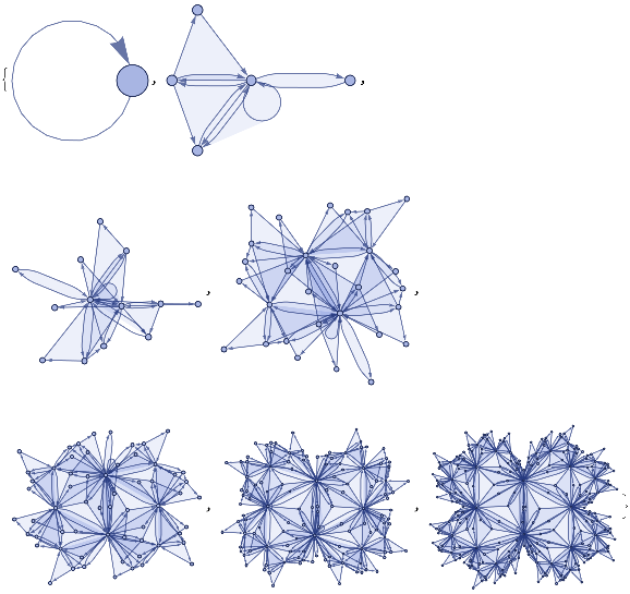
Below is the case for absolute continuity, that we will use, going forward.
ResourceFunction["WolframModelPlot"][#,VertexLabels->Automatic]&/@ResourceFunction["WolframModel"][{{a,b}}->{{a,c},{c,b},{b,e,a},{d,f,a},{a,d,b},{a,b,c},{a,d,c}},{{0,0}},3,"StatesList"]
Out[]=
ResourceFunction["WolframModelPlot"][#,VertexLabels->None]&/@ResourceFunction["WolframModel"][{{a,b}}->{{a,c},{c,b},{b,e,a},{d,f,a},{a,d,b},{a,b,c},{a,d,c}},{{0,0}},6,"StatesList"]
Out[]=
1.2 Rule Evolutions -Maintaining Space
1.2 Rule Evolutions -Maintaining Space
One can think of a causal graph as representing causal relationships in both space and time. Successive events or nodes define chronology. When dealing with large connections of nodes, the clusters and neighbourhoods provide more information than their position in the generated graph . A multiway system deals with multiple paths of history and multiple generation procedures .
Using the Wolfram model, one can translate these rules to a Hypergraph. In this formal, algebraic representation of discrete spatial relation, one must identify whether the relations remain logically consistent. The set substitution rule created can be used to transform a Hypergraph. Due to the lack of specific updating order,the evolution of this spatial hypergraph will be non-deterministic.
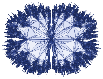
Idealiseduniverse=ResourceFunction["WolframModel"][{{a,b}}->{{a,c},{c,b},{b,e,a},{d,f,a},{a,d,b},{a,b,c},{a,d,c}},{{0,0}},11,"FinalStatePlot"]
Out[]=
1.2 Identifying Curvature and approximate Dimension
1.2 Identifying Curvature and approximate Dimension
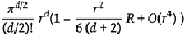
Here one must consider the geometric projection of Ricci Curvature.This is done by picking a vertex and attempting to find the shortest path to another vertex in the graph arrangement. The volume spanned by both the tubes representing the edge traversal procedure, and the set of possible paths, allows for curvature to be approximated. We use the correction volume of this pseudo-hyperbolic surface as a means to Calculate the Ricci Curvature R in (2)
idealisedUniverseGraphForm=ResourceFunction["HypergraphToGraph"][ResourceFunction["WolframModel"][{{a,b}}{{a,c},{c,b},{b,e,a},{d,f,a},{a,d,b},{a,b,c},{a,d,c}},{{0,0}},8,"FinalState"]]
Out[]=
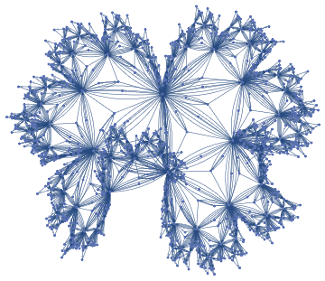
In this above case, a non dimension-specific visualisation of the discreteness rule was created.
In[]:=
1.3 Emerging Curvature
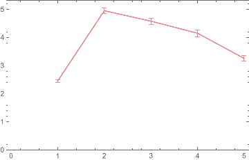
VolumeList[g_Graph,v_]:=N[First[Values[ResourceFunction["GraphNeighborhoodVolumes"][g,{v}]]]];ricciGraph=Graph[ResourceFunction["HypergraphToGraph"][ResourceFunction["WolframModel"][{{a,b}}{{a,c},{c,b},{b,e,a},{d,f,a},{a,d,b},{a,b,c},{a,d,c}},{{0,0}},11,"FinalState"]],VertexStyle->ResourceFunction["WolframPhysicsProjectStyleData"]["SpatialGraph","VertexStyle"],EdgeStyle->ResourceFunction["WolframPhysicsProjectStyleData"]["SpatialGraph","EdgeLineStyle"]];With[{u=VolumeList[ricciGraph,#]&/@{385,3041}},ListLinePlot[Transpose[{Range[Length[#]]-1,#}]&/@u,Mesh->All,Frame->True,PlotRange->{0,Max[u]+1},PlotStyle->ResourceFunction["WolframPhysicsProjectStyleData"]["GenericLinePlot","PlotStyles"]]]
Out[]=
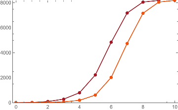
Looking at growth rates of volumes in the limit of 10 steps, we can measure the volumes of the tubes like to compute approximations to projections of the Ricci Curvature in this universal model models.
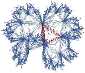
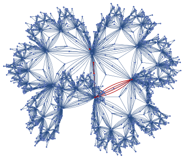
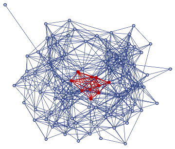
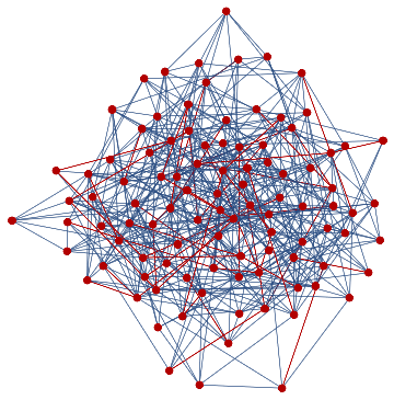
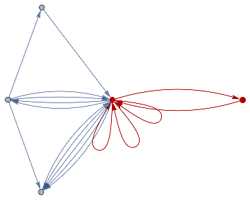
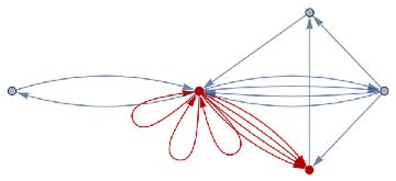
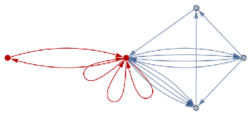
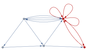
finalState=ResourceFunction["WolframModel"][{{a,b}}{{a,c},{c,b},{b,e,a},{d,f,a},{a,d,b},{a,b,c},{a,d,c}},{{0,0}},8,"FinalState"];toHighlight=Function[r,Catenate@Through[{Join[List@@@#,List@@@Reverse/@#]&@*EdgeList,VertexList}[With[{graph=ResourceFunction["HypergraphToGraph"][ResourceFunction["WolframModel"][{{a,b}}{{a,c},{c,b},{b,e,a},{d,f,a},{a,d,b},{a,b,c},{a,d,c}},{{0,0}},8,"FinalState"]]},GraphUnion@@(NeighborhoodGraph[graph,#,r]&/@FindShortestPath[graph,200,900])]]]]/@{1,3};ResourceFunction["WolframModelPlot"][finalState,EdgeStyle-><|Alternatives@@#->Directive[Thick,Red]|>,VertexStyle-><|Alternatives@@#->Directive[Thick,Red]|>]&/@toHighlight
Out[]=
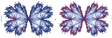
This is the case of positive curvature above where the red points represent small tubes. Considering Hypergraph neighbourhood volumes , one can estimate the Dimension of a Hypergraph:
HypergraphDimensionEstimateList[hg_]:=ResourceFunction["LogDifferences"][MeanAround/@Transpose[Values[ResourceFunction["HypergraphNeighborhoodVolumes"][hg,All,Automatic]]]];ListLinePlot[HypergraphDimensionEstimateList[List@@@EdgeList[Graph3D[ResourceFunction["HypergraphToGraph"][ResourceFunction["WolframModel"][{{a,b}}{{a,c},{c,b},{b,e,a},{d,f,a},{a,d,b},{a,b,c},{a,d,c}},{{0,0}},8,"FinalState"]]]]],Frame->True,PlotStyle->ResourceFunction["WolframPhysicsProjectStyleData"]["GenericLinePlot","PlotStyles"],PlotRange->{0,Automatic}]
Out[]=
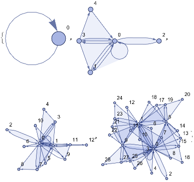
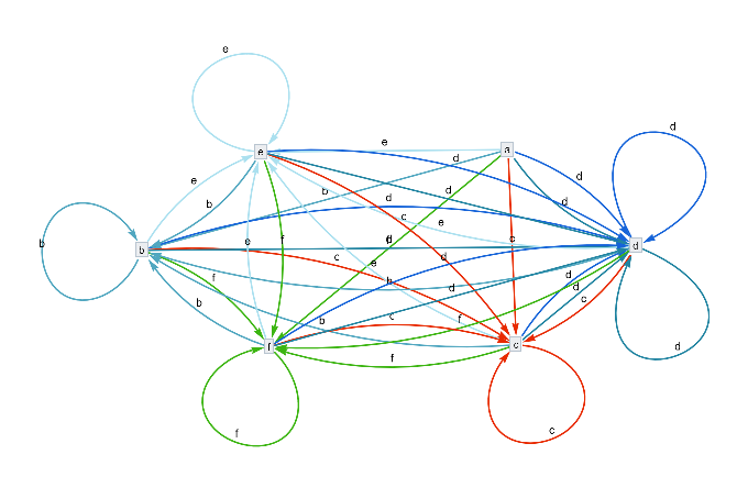
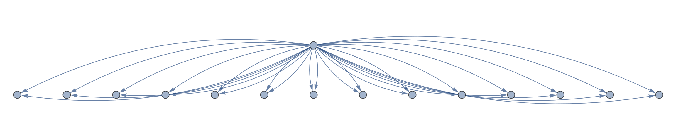
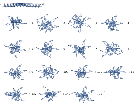
The nest graph for the potential substitutions , representing the various positions within the above Universal model .
ResourceFunction["NestGraphTagged"][a{c,d,f,e,b,d},a,2,EdgeLabels->(DirectedEdge[_,_,i_]:>Placed[Text@({"c","d","f","e","b","d"}[[i]]),0.5]),AspectRatio->.4,"StateLabeling"->True,"FormattingFunction"->(Style[Text[#],9,Black]&),FormatTypeStandardForm,ImageSize->680]
Out[]=
2.Checking Graph rewriting systems
2.Checking Graph rewriting systems
This section involves checking ordinary graph rewriting systems first, using the IGraphM Library to find sub - isomorphisms, count those sub-isomorphisms and analyze the frequencies of certain subgraph motifs .
Graphs provide an expressive means to represent evolution. It follows that a graph-rewriting rule should be applied to the Universe generated above to identify the range of all possible generations . The aim is to replace one subgraph with another. The sequential rewriting computes one subgraph at a time. The multiway system of this rewrite looks at the dependency of these rules and analyzes the computational, non-deterministic decision of subgraph attachment [4]
Here we used the number of applicable hypergraph rewrites in order to assess homogeneity.
It is important to note that, for hypergraphs, one would need to convert the hypergraphs to graphs and Check for Sub-Isomorphisms.
2.1 Sub-isomorphisms and Counting
2.1 Sub-isomorphisms and Counting
This kind of bijection is commonly described as "edge-preserving bijection", in accordance with the general notion of isomorphism being a structure - preserving bijection.
First we retrieve the IGraph Library
<<IGraphM`
Out[]=
IGraph/M 0.5.1 (October 12, 2020) |
Evaluate |
Unofficial fast - directed - graph rewriting code
Unofficial fast - directed - graph rewriting code
Many thanks to Yorick Zeschke for helping me with this section.
In[]:=
loopsToColourSpec[directedGraph_]:=Normal[Diagonal[AdjacencyMatrix[directedGraph]]]removeIlicitEdges[V_,E_]:=Graph[V,DeleteCases[If[ContainsAll[V,{#[[1]],#[[2]]}],#,Null]&/@E,Null],VertexLabelsAll]rewriteStep[L_,R_,G_]:=Module[{el=EdgeList[L],vl=VertexList[L],vg=VertexList[G],eg=EdgeList[G],er=EdgeList[R],vr=VertexList[R]},vr=vr/.Thread[##+VertexCount[G]]&[Complement[vr,vl]];Counts[CanonicalGraph[removeIlicitEdges[Union[Complement[vg,vl/.#],vr/.#],Union[Complement[eg,el/.#],er/.#]]]&/@IGVF2FindSubisomorphisms[{SimpleGraph[L],"VertexColors"loopsToColourSpec[L]},{SimpleGraph[G],"VertexColors"loopsToColourSpec[G]}]]]rewriteStep[rules_List,init_Graph]:=Merge[rewriteStep[#[[1]],#[[2]],init]&/@rules,Total]rewriteProbs[rules_List,init_Graph]:=#/If[Total[Values[#]]0,1,Total[Values[#]]]&[rewriteStep[rules,init]]randomMultiwayPath[rules_,init_,0_]:={}randomMultiwayPath[rules_,init_,steps_]:=Prepend[randomMultiwayPath[rules,#,steps-1],#]&[RandomChoice[(Values[#]Keys[#])&[rewriteProbs[rules,init]]]]rewriteMultiway[rules_,init_,steps_]:=Module[{graph=DirectedGraph[{}],leaves={init},newEdges},For[i=1,i≤steps,i+=1,newEdges=Flatten[Function[s,Function[r,DirectedEdge[s,#[[1]],{r[[2]],#[[2]]}]&/@Normal[rewriteStep[r[[1,1]],r[[1,2]],s]]]/@Thread[rulesRange[Length[rules]]]]/@leaves,2];graph=GraphUnion[graph,DirectedGraph[newEdges]];leaves=DeleteDuplicates[newEdges[[;;,2]]]];graph]multiwayPlot[g1_]:={Graph[g1,VertexLabelsThread[VertexList[g1]Range[VertexCount[g1]]]],Thread[(GraphPlot[#,GraphLayout"SpringElectricalEmbedding",ImageSize100]&/@VertexList[g1])Range[VertexCount[g1]]]}inj[F_,G_]:=Length[IGVF2FindSubisomorphisms[{SimpleGraph[F],"VertexColors"loopsToColourSpec[F]},{SimpleGraph[G],"VertexColors"loopsToColourSpec[G]}]]
The basic problem is to start from two graphs (or hypergraphs), with vertex sets V1 and V2 and edge sets E1 and E2, and construct a function f that maps between V1 and V2 in such a way as to maximise the number of edges in E1 mapped to edges in E2 . The proportion of edges in E1 mapped to edges in E2 is effectively the "degree of approximation" of the map.
In[]:=
atest=ResourceFunction["HypergraphToGraph"][ResourceFunction["WolframModel"][{{a,b}}{{a,c},{c,b},{b,e,a},{d,f,a},{a,d,b},{a,b,c},{a,d,c}},{{0,0}},8,"FinalState"]];
In[]:=
btest=EdgeAdd[CycleGraph[5],3<->4];
In[]:=
atestdirect=DirectedGraph[ResourceFunction["HypergraphToGraph"][ResourceFunction["WolframModel"][{{a,b}}{{a,c},{c,b},{b,e,a},{d,f,a},{a,d,b},{a,b,c},{a,d,c}},{{0,0}},8,"FinalState"]],"Random"];
In[]:=
btestdirect=DirectedGraph[EdgeAdd[CycleGraph[5],3<->4]];
If one wants to maximise the number of edges that get mapped from G1 into G2, mappings of all possible vertices from G1 into G2 (assuming G2 has at least as many vertices as G1) and select those with the most preserved edges. The vertices count can be ensured by sorting.
HighlightGraph[atest,Subgraph[atest,btest]]
Out[]=
In[]:=
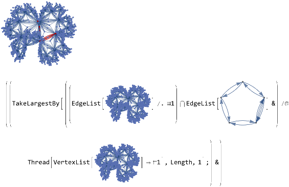
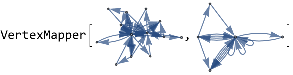
vertexMapper[G1_,G2_]:=Module[{mappings=Thread[VertexList[G1]->#]&/@Flatten[Permutations/@Subsets[VertexList[G2],{VertexCount[G1]}],1]},TakeLargestBy[Intersection[EdgeList[G1]/.#,EdgeList[G2]]&/@Thread[VertexList[G1]->#],Length,1];&HighlightGraph[G1,G2]]
vertexMapper[atestdirect,btestdirect]
Out[]=
vertexMapper[atest,btest]
Out[]=

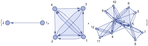
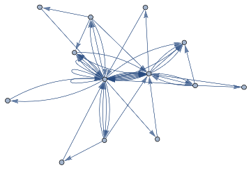
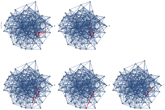
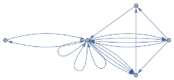
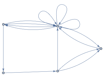
mwtest=ResourceFunction["MultiwaySystem"]["WolframModel"->{{{a,b}}->{{a,c},{c,b},{b,e,a},{d,f,a},{a,d,b},{a,b,c},{a,d,c}}},{{{0,0}}},2,"EvolutionEventsGraph",VertexSize->1]
Out[]=
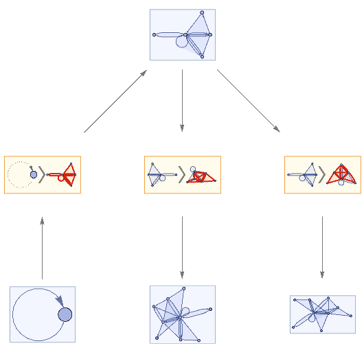
Evolving the multiway system for one step has resulted in three possible configurations. This tells us that there are three subhypergraphs of the universe Hypergraph representation are isomorphic to the Hypergraph itself. This is a homogeneity assessments calculable in both graphs and hypergraphs without first needing to implement a full subgraph isomorphism algorithm.
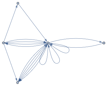
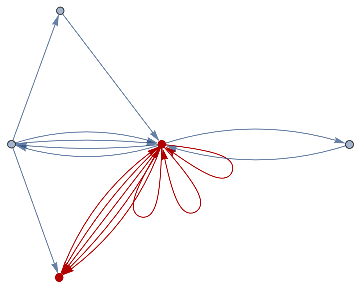
rewritetest=rewriteMultiway[Graph[{12,23,34}]Graph[{12,23,34,4->1}],ResourceFunction["HypergraphToGraph"][ResourceFunction["WolframModel"][{{a,b}}{{a,c},{c,b},{b,e,a},{d,f,a},{a,d,b},{a,b,c},{a,d,c}},{{0,0}},2,"FinalState"]],1]
Out[]=
multiwayPlot[rewritetest]
Out[]=
In[]:=
AnalyzingmotifsandcliquesinthegeneratedUniverse
The aim is to modify an arbitrary graph by removing or adding edges, based on already present connectivity as well as to find different approximately similar forms of the same subgraph and group them together such that they can be compared (as a group representing a specific approximate subgraph) against regions of a large graph (a spatial hypergraph for example) to test for the approximate isomorphism . This approach is an attempt to solve the efficiency problem that arises from checking each vertex (for similar vertex information such as the same vertex degree or neighborhood) in the large graph and looking for the counts of different subgraphs . This is similar to a very rough goodness - of - fit test for differing subgraph distributions . This would be a powerful measure for subgraphs mapping onto larger graphs .
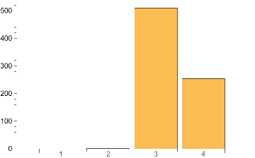
Using functions for finding or counting all complete subgraphs of a graph, I can identify methods of finding the most recurring subgraph .
IGMaximalCliqueSizeCounts[atest]BarChart[%,ChartLabels->Range@Length[%]]
Out[]=
{0,1,510,254}
Out[]=
IGMotifsTotalCount[atest,4]
Out[]=
288080
IGMotifsTotalCount[atest,3]
Out[]=
22181
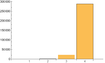
Table[IGMotifsTotalCount[atest,i],{i,4}]BarChart[%,ChartLabels->Range@Length[%]]
Out[]=
{0,1274,22181,288080}
Out[]=
Floor[VertexCount[atest]/16]
Out[]=
63
ResourceFunction["HypergraphToGraph"][ResourceFunction["WolframModel"][{{a,b}}{{a,c},{c,b},{b,e,a},{d,f,a},{a,d,b},{a,b,c},{a,d,c}},{{0,0}},2,"FinalState"]]
Out[]=
VertexMapper[ResourceFunction["HypergraphToGraph"][ResourceFunction["WolframModel"][{{a,b}}{{a,c},{c,b},{b,e,a},{d,f,a},{a,d,b},{a,b,c},{a,d,c}},{{0,0}},2,"FinalState"]],ResourceFunction["HypergraphToGraph"][ResourceFunction["WolframModel"][{{a,b}}{{a,c},{c,b},{b,e,a},{d,f,a},{a,d,b},{a,b,c},{a,d,c}},{{0,0}},1,"FinalState"]]]
Out[]=
mappings=Thread[VertexList[ResourceFunction["HypergraphToGraph"][ResourceFunction["WolframModel"][{{a,b}}{{a,c},{c,b},{b,e,a},{d,f,a},{a,d,b},{a,b,c},{a,d,c}},{{0,0}},2,"FinalState"]]]->#]
Out[]=
{0#1,2#1,3#1,4#1,1#1,5#1,6#1,7#1,8#1,9#1,10#1,11#1,12#1}
Now we must generate a test for the predictable case:
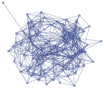
ControlCase=ResourceFunction["FlatManifoldToGraph"][4,0.5,100]["SpatialGraph"]
Out[]=
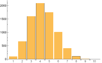
IGCliqueSizeCounts[ControlCase]BarChart[%,ChartLabels->Range@Length[%]]
Out[]=
{100,663,1601,2091,1753,1019,410,107,16,1}
Out[]=
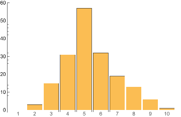
IGMaximalCliqueSizeCounts[ControlCase]BarChart[%,ChartLabels->Range@Length[%]]
Out[]=
{0,3,15,31,57,32,19,13,6,1}
Out[]=
IGMotifsTotalCount[ControlCase,3]
Out[]=
6472
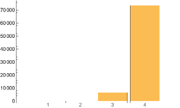
Table[IGMotifsTotalCount[ControlCase,i],{i,4}]BarChart[%,ChartLabels->Range@Length[%]]
Out[]=
{0,90,6472,73615}
Out[]=
FindClique[ControlCase]
Out[]=
{{{0.427957,0.371315,0.122219,0.160984},{0.305591,0.279899,0.34459,0.523553},{0.375976,0.309613,0.250314,0.117958},{0.410904,0.27795,0.450923,0.402835},{0.394253,0.127345,0.36112,0.417581},{0.408239,0.0551439,0.240724,0.109069},{0.375314,0.188195,0.367831,0.142999},{0.336482,0.309272,0.169543,0.257877},{0.180135,0.287137,0.343917,0.389793},{0.56982,0.0604439,0.311702,0.184353}}}
HighlightGraph[ControlCase,Subgraph[ControlCase,%]]
Out[]=
FindClique[ControlCase,Infinity,All];HighlightGraph[ControlCase,Subgraph[ControlCase,%]]
Out[]=
FindClique[atest];HighlightGraph[atest,Subgraph[atest,%]]
Out[]=
Testing the distribution from a random function.
RandomGraph[BernoulliGraphDistribution[100,0.1]]
Out[]=
FindClique[RandomGraph[BernoulliGraphDistribution[100,0.1]]];HighlightGraph[RandomGraph[BernoulliGraphDistribution[100,0.1]],Subgraph[RandomGraph[BernoulliGraphDistribution[100,0.1]],%]]
Out[]=
FindClique[RandomGraph[BernoulliGraphDistribution[100,0.1]],Infinity,All];HighlightGraph[RandomGraph[BernoulliGraphDistribution[100,0.1]],Subgraph[RandomGraph[BernoulliGraphDistribution[100,0.1]],%]]
Out[]=
In[]:=
g=RandomGraph[BernoulliGraphDistribution[100,0.1]];
Table[HighlightGraph[g,Subgraph[g,clique]],{clique,FindClique[g,Infinity,5]}]
Out[]=
Approximate Isomorphism
Approximate Isomorphism
Given two graphs G1, G2, we are interested in finding a bijection from V (G1) to V (G2) that maximizes the number of complete edge mappings (where V is the set of vertices) . This edge preserving bijection is an NP - Hard problem and is considered a problem unlikely to ever be NP - complete . Considering alternate rounding procedures[5], one can come to the conclusion that the more extreme structures must be retained in order to preserve the structural information of the graph network itself .
Direct subgraph Isomorphism checking
Direct subgraph Isomorphism checking
This code uses a brute force approach to check neighbourhoods of graphs and identify Statistical Uniformity using graph network geodesics.
In[]:=
matrixPermute[M_,p_]:=Table[M[[p[[i]],p[[j]]]],{i,1,Length[M]},{j,1,Length[M]}](*assumingsquare*)distSameNumNodes[G_,H_]:=Min[Norm[AdjacencyMatrix[G]-matrixPermute[AdjacencyMatrix[H],#]]&/@Permutations[Range[VertexCount[H]]]]allSubgraphDistances[G_,H_]:=Min[distSameNumNodes[Subgraph[G,#],H]&/@Subsets[VertexList[G],{VertexCount[H]}]]+(VertexCount[G]-VertexCount[H])+(EdgeCount[G]-EdgeCount[H])(*assumingGhasmorenodes*)graphDistance[G_,H_]:=Piecewise[{{distSameNumNodes[G,H],VertexCount[G]==VertexCount[H]},{allSubgraphDistances[G,H],VertexCount[G]>VertexCount[H]},{allSubgraphDistances[H,G],VertexCount[G]<VertexCount[H]}}]pairWiseDist[G_]:=Module[{pairs=Subsets[VertexList[G],{2}]},graphDistance[NeighborhoodGraph[G,#[[1]],1],NeighborhoodGraph[G,#[[2]],1]]&/@pairs[[;;5]]]StatisticalUniformity[G_]:=Mean[pairWiseDist[G]]
G=DirectedGraph[ResourceFunction["HypergraphToGraph"][ResourceFunction["WolframModel"][{{a,b}}{{a,c},{c,b},{b,e,a},{d,f,a},{a,d,b},{a,b,c},{a,d,c}},{{0,0}},1,"FinalState"]]]
Out[]=
pairWiseDist[G]
Out[]=
{6,15,3,10,10}
StatisticalUniformity[G]
Out[]=
44
5
This is the function for perturbing the graph/ subgraph structures:
In[]:=
GraphPerturbation[g_Graph]:=Module[{degrees=VertexDegree[g],weights,randomPositivePair,randomNegativePair},weights=Catenate@Outer[Plus,degrees,degrees];randomPositivePair=RandomChoice[weights->Tuples[VertexList[g],2]];randomNegativePair=RandomChoice[1/(1+weights)->Tuples[VertexList[g],2]];EdgeAdd[EdgeDelete[g,EdgeList[g,_@@randomPositivePair]],DirectedEdge@@randomNegativePair]]
UniverseTest=DirectedGraph[ResourceFunction["HypergraphToGraph"][ResourceFunction["WolframModel"][{{a,b}}{{a,c},{c,b},{b,e,a},{d,f,a},{a,d,b},{a,b,c},{a,d,c}},{{0,0}},1,"FinalState"]]]
Out[]=
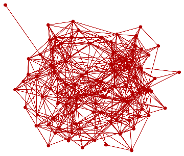
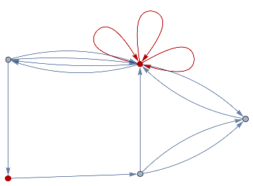
IGCliqueSizeCounts[UniverseTest];IGCliqueSizeCounts0=BarChart[%,ChartLabels->Range@Length[%]];IGMaximalCliqueSizeCounts[UniverseTest];IGMaximalCliqueSizeCounts0=BarChart[%,ChartLabels->Range@Length[%]];Table[IGMotifsTotalCount[UniverseTest,i],{i,4}];IGMotifsTotalCountTable0=BarChart[%,ChartLabels->Range@Length[%]];FindClique[UniverseTest]HighlightGraph[UniverseTest,Subgraph[UniverseTest,%]]
Out[]=
{{0,1}}
Out[]=
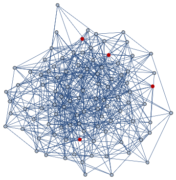
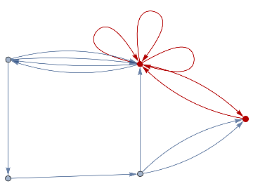
perturbedgraph1=GraphPerturbation[UniverseTest]
Out[]=
In[]:=
FindClique[perturbedgraph1]HighlightGraph[UniverseTest,Subgraph[UniverseTest,%]]
Out[]=
{{0,2}}
Out[]=
FindClique[UniverseTest]HighlightGraph[perturbedgraph1,Subgraph[perturbedgraph1,%]]
Out[]=
{{0,1}}
Out[]=
IGCliqueSizeCounts[perturbedgraph1];IGCliqueSizeCounts1=BarChart[%,ChartLabels->Range@Length[%]];IGMaximalCliqueSizeCounts[perturbedgraph1];IGMaximalCliqueSizeCounts1=BarChart[%,ChartLabels->Range@Length[%]];Table[IGMotifsTotalCount[perturbedgraph1,i],{i,4}];IGMotifsTotalCountTable1=BarChart[%,ChartLabels->Range@Length[%]];FindClique[perturbedgraph1]HighlightGraph[perturbedgraph1,Subgraph[perturbedgraph1,%]]
Out[]=
{{0,2}}
Out[]=
perturbedgraph2=GraphPerturbation[perturbedgraph1];FindClique[perturbedgraph2]HighlightGraph[UniverseTest,Subgraph[UniverseTest,%]]
Out[]=
{{0,2}}
Out[]=
FindClique[UniverseTest];HighlightGraph[perturbedgraph2,Subgraph[perturbedgraph2,%]];IGCliqueSizeCounts[perturbedgraph2];IGCliqueSizeCounts2=BarChart[%,ChartLabels->Range@Length[%]];IGMaximalCliqueSizeCounts[perturbedgraph2];IGMaximalCliqueSizeCounts2=BarChart[%,ChartLabels->Range@Length[%]];Table[IGMotifsTotalCount[perturbedgraph2,i],{i,4}];IGMotifsTotalCountTable2=BarChart[%,ChartLabels->Range@Length[%]];FindClique[perturbedgraph2];HighlightGraph[perturbedgraph2,Subgraph[perturbedgraph2,%]]
Out[]=
perturbedgraph3=GraphPerturbation[perturbedgraph2]
Out[]=
FindClique[perturbedgraph3];HighlightGraph[UniverseTest,Subgraph[UniverseTest,%]];FindClique[UniverseTest]HighlightGraph[perturbedgraph3,Subgraph[perturbedgraph3,%]]
Out[]=
{{0,1}}
Out[]=
IGCliqueSizeCounts[perturbedgraph3];IGCliqueSizeCounts3=BarChart[%,ChartLabels->Range@Length[%]];IGMaximalCliqueSizeCounts[perturbedgraph3];IGMaximalCliqueSizeCounts3=BarChart[%,ChartLabels->Range@Length[%]];Table[IGMotifsTotalCount[perturbedgraph3,i],{i,4}];IGMotifsTotalCountTable3=BarChart[%,ChartLabels->Range@Length[%]];FindClique[perturbedgraph3]HighlightGraph[perturbedgraph3,Subgraph[perturbedgraph3,%]]
Out[]=
{{0,2}}
Out[]=
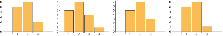
Below shows the change in Clique size counts after 3 successive perturbations . The cliques structures are maintained .
Grid[{{IGCliqueSizeCounts0,IGCliqueSizeCounts1,IGCliqueSizeCounts2,IGCliqueSizeCounts3}}]
Out[]=
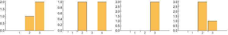
Below shows the change in the Maximal Clique size counts after 3 successive perturbations . The Maximal cliques structures are maintained .
Grid[{{IGMaximalCliqueSizeCounts0,IGMaximalCliqueSizeCounts1,IGMaximalCliqueSizeCounts2,IGMaximalCliqueSizeCounts3}}]
Out[]=
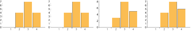
Below shows the change in Total counts of motifs of Vertex count 1-4 , after 3 successive perturbations . The motif structures are also maintained .
Grid[{{IGMotifsTotalCountTable0,IGMotifsTotalCountTable1,IGMotifsTotalCountTable2,IGMotifsTotalCountTable3}}]
Out[]=
perturbedgraph4=GraphPerturbation[perturbedgraph3];perturbedgraph5=GraphPerturbation[perturbedgraph4];perturbedgraph6=GraphPerturbation[perturbedgraph5];perturbedgraph7=GraphPerturbation[perturbedgraph6];perturbedgraph8=GraphPerturbation[perturbedgraph7];
SU0=StatisticalUniformity[perturbedgraph1];SU1=StatisticalUniformity[perturbedgraph2];SU2=StatisticalUniformity[perturbedgraph3];SU3=StatisticalUniformity[perturbedgraph4];SU4=StatisticalUniformity[perturbedgraph5];SU5=StatisticalUniformity[perturbedgraph6];SU6=StatisticalUniformity[perturbedgraph7];SU7=StatisticalUniformity[perturbedgraph8];
Grid[{{ListPlot[{{SU0,SU1,SU2,SU3,SU4,SU5,SU6,SU7}},Filling->Axis],ListLinePlot[{{SU0,SU1,SU2,SU3,SU4,SU5,SU6,SU7}},Filling->Axis]}}]
Out[]=
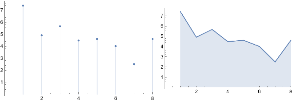
As we make the graph isomorphism more and more approximate, what effect does that have?
The answer is that statistical uniformity decreases as evident in the above plot. Plotting more values would permit a more logically consistent conclusion regarding statistical uniformity.
The answer is that statistical uniformity decreases as evident in the above plot. Plotting more values would permit a more logically consistent conclusion regarding statistical uniformity.
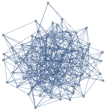
UniverseTest=DirectedGraph[ResourceFunction["HypergraphToGraph"][ResourceFunction["WolframModel"][{{a,b}}{{a,c},{c,b},{b,e,a},{d,f,a},{a,d,b},{a,b,c},{a,d,c}},{{0,0}},8,"FinalState"]]]
Out[]=
In[]:=
perturbedgraph1=GraphPerturbation[UniverseTest];perturbedgraph2=GraphPerturbation[perturbedgraph1];perturbedgraph3=GraphPerturbation[perturbedgraph2];perturbedgraph4=GraphPerturbation[perturbedgraph3];perturbedgraph5=GraphPerturbation[perturbedgraph4];perturbedgraph6=GraphPerturbation[perturbedgraph5];perturbedgraph7=GraphPerturbation[perturbedgraph6];perturbedgraph8=GraphPerturbation[perturbedgraph7];
a10=IGMotifsTotalCountEstimate[UniverseTest,3,10];a11=IGMotifsTotalCountEstimate[perturbedgraph1,3,10];a12=IGMotifsTotalCountEstimate[perturbedgraph2,3,10];a13=IGMotifsTotalCountEstimate[perturbedgraph3,3,10];a14=IGMotifsTotalCountEstimate[perturbedgraph4,3,10];a15=IGMotifsTotalCountEstimate[perturbedgraph5,3,10];a16=IGMotifsTotalCountEstimate[perturbedgraph6,3,10];a17=IGMotifsTotalCountEstimate[perturbedgraph7,3,10];a18=IGMotifsTotalCountEstimate[perturbedgraph8,3,10];
Grid[{{ListPlot[{{a10,a11,a12,a13,a14,a15,a16,a17,a18}},Filling->Axis,PlotStyleRed],ListLinePlot[{{a10,a11,a12,a13,a14,a15,a16,a17,a18}},Filling->Axis,PlotStyleRed]}}]
Out[]=
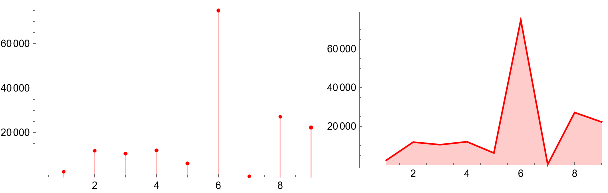
The computation of mapping sub hypergraphs to approximately isomorphic subhypergraphs must be made such that the permutations cover as much of the space as possible while limiting overlaps.
The question is what kind of computation this corresponds to in the continuous case?This is an open question.
The question is what kind of computation this corresponds to in the continuous case?This is an open question.
Statistically Uniform Regions of the Spatial Hypergraph - The Vacuum
Statistically Uniform Regions of the Spatial Hypergraph - The Vacuum
From the plots it can be identified that, across perturbations, communities such as cliques and motifs remain consistent . By making the isomorphism more approximate, by locating cliques within perturbations and drawing a comparison with the initial, unperturbed state, one can attempt to find a method of formulating a method to identify Statistical Uniformity. By Analysing neighborhood graphs that span a Euclidean distance of 1 node away from the random node being analyzed, an approximation of Uniformity can be considered .
It is clear that Statistical Uniformity actually DECREASES as the graph is perturbed. This is extremely predictable, and equally as interesting. The question that follows is, what value does this tend to at the limit of perturbations? I could not find an explicit answer due to reaching the recursion limit, which means future iterations on this approach would require a modification to the number of subgraphs and regions being checked for neighbourhood relations, or (alternatively) the region checking calculation itself.
It is clear that Statistical Uniformity actually DECREASES as the graph is perturbed. This is extremely predictable, and equally as interesting. The question that follows is, what value does this tend to at the limit of perturbations? I could not find an explicit answer due to reaching the recursion limit, which means future iterations on this approach would require a modification to the number of subgraphs and regions being checked for neighbourhood relations, or (alternatively) the region checking calculation itself.
Concluding remarks
Concluding remarks
The work so far was extremely encouraging, but is not yet finished.
There is still some fascinating work left to carry out in order to complete the case for forming analogues to the Vacuum in this discrete computational representation of a Continuous universe.
future steps would need to be highlighted below.
There is still some fascinating work left to carry out in order to complete the case for forming analogues to the Vacuum in this discrete computational representation of a Continuous universe.
future steps would need to be highlighted below.
◼
Re-program the statistical uniformity function to include graph perturbations as a parameter.
◼
Run the Statistical uniformity for a larger hypergraph (after making the program more computationally efficient).
◼
Tangentially, find a set of common subgraphs within the Universal structure, perturb them using the graph perturbation function a number of times , then map them onto the initial Universe plot. See if there can be any trends that relate motif size to clique size. This would provide an undeniable argument of localised structure preservation.
◼
Run this analysis on the Wolfram Model Registry universes, once optimised.
Keywords
Keywords
◼
Graph Isomorphism problem
◼
Discrete mathematics
◼
Computational Complexity
Acknowledgment
Acknowledgment
I would like to thank my Mentor, Jonathan Gorard, for setting me up with this incredible challenge of finding statistical uniformities in discrete and abstract systems such as these. I would like to thank Yorick Zeschke for his incredible insight and guidance as well as his programming assistance. I would also like to thank Xerxes Arsiwalla, Hatem Elshatlawy and the members of my group during this Winter School for their continued support. Last but not least, I would also like to thank Stephen Wolfram for helping with the progression of this project by providing valuable methods to approach the task of Statistical Uniformity Identification, during our various engaging discussions and conversations.
References
References
◼
[2]L. Livi and A. Rizzi. 2013. The Graph Matching Problem. Pattern Analysis and Application 16 (2013), 253–283
◼
[3]Scheinerman, Edward; Ullman, Daniel (December 20, 2013). Fractional Graph Theory. Dover Publications. ISBN 978-0486485935.
Categories: Graph theory
Categories: Graph theory
◼
[4]Blostein, Dorothea & Fahmy, Hoda & Grbavec, Ann. (1995). Practical Use of Graph Rewriting
◼
[5]Sanjeev Arora, Alan M. Frieze, and Haim Kaplan. A new rounding procedure for the assignment problem with applications to dense graph arrangement problems. Math. Program., 92(1):1–36, 2002