ARTICLE (original article): Approximate mathematical treatments are commonly taught in undergraduate chemistry, but the validity ranges of these approximations have rarely been properly defined. We present error contour plots of commonly used quadratic approximations for calculating equilibrium proton concentrations of monoprotic acids. Students and instructors can easily read these plots to estimate the error in their approximation of proton concentration (1%, 5%, 10%, and 25%) at a given initial acid concentration and dissociation constant value. In addition, we introduce a new quadratic expression which will always deliver an error no larger than 25% (or 0.1 pH unit) in ideal solution irrespective of the acid strength and concentration. These results extend readily to their analogue of pOH, , and for bases. Our novel approach here could significantly reduce many different situations students must master into one that can be computed straightforwardly without caveats or conditions. CITATION (original article): Limpanuparb, T.; Ho J. (2023), Visualization of Validity Ranges for Acid Approximations: Error Contour Plots as a Function of Concentration and .https://doi.org/10.1021/acs.jchemed.3c00751
[HA]
0
K
a
K
b
[
-
A
]
K
a
Introduction
Introduction
To obtain the exact solution for the pH of a monoprotic acid solution, the following cubic equation is to be solved.
3
[]
+
H
2
K
a
+
H
K
a
0
K
w
+
H
K
a
K
w
(
1
)[HA]
0
K
a
K
w
As solving this cubic equation can be quite complex, different approximation methods are presented in textbooks and articles to reduce this equation into simpler quadratic forms. The following are three common methods .
1
.Direct substitution: quadratic equation derived from the “Reaction Initial Change Equilibrium” table, neglecting effects of self-ionization of water
2
.Simple square root: square root equation simplified from the quadratic equation in method 1, neglecting effects of self-ionization of water and change in acid concentration
3
.Handerson-Hasselbalch equation (HH-like): equation for buffer solutions, assuming the concentration of acid and its salt are constant at equilibrium and neglecting effects of self-ionization of water
The following equilibrium constant expression derived in the article “Acid-Base Approximations in Ideal Solution Revisited: Error Contour Plots as a Function of and Acid Concentration” (Limpanuparb & Ho, 2023) can lead to different approximations by replacing one term or both terms in red with a constant.
K
a
[][]-
+
H
+
H
K
w
[]
+
H
[HA]
0
+
H
K
w
[]
+
H
(
2
)The lower bound and upper bound values of the term in red are 0 and , respectively (see details in the article). This program explores the three approximation methods using 0, or in place of the terms in red. The terms in the numerator and denominator are replaced independently, resulting in 9 possible equations for each approximation method. The term replacements can result in the same equations among different approximation methods. Removing duplicates in the 9 x 3 = 27 possible equations results in 18 unique approximation equations. The initialization section in the source code of the programs lists out the 18 approximation equations and the exact (cubic) equation, totalling to 19 equations. Variable names for these equations represent the approximation method (x1, x2, x3 for method 1, 2 and 3, respectively) and term replacements in the numerator and the denominator (0, r, w for 0, ,, respectively). For example, equation x1wr represents a direct substitution equation using as the red term in the numerator and as the red term in the denominator. The equation is displayed in its polynomial form as +(+)[]-[HA]++=0.
K
w
K
w
K
w
[]
+
H
K
w
K
w
[]
+
H
K
w
[]
+
H
K
w
2
[]
+
H
K
a
[]
-
A
0
+
H
K
a
0
K
w
K
a
K
w
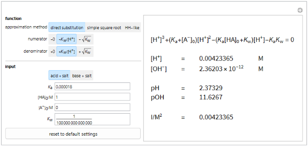
Calculation of pH
Calculation of pH
This program calculates the concentration of hydronium and hydroxide ions, pH and pOH from input values of ,, , and . and are real numbers greater than 0, while , and are real numbers greater than or equal to 0. If a value outside of this range is entered, the program will automatically revert it back to the corresponding default value.
The acid + salt mode uses approximation equations explained in the introduction, while the base + salt mode uses the same equations, but replacing with , with [] and switching [HA] and ]. If the calculated value for in acid + salt mode or []in base + salt mode is greater than 0, then the output box will display the calculated values for , [], pH, pOH and ionic strength (I). Otherwise, the message “This formula is not applicable to the input.” will be shown.
K
a
K
w
[HA]
0
[]
-
A
0
K
a
K
w
[HA]
0
[]
-
A
0
The acid + salt mode uses approximation equations explained in the introduction, while the base + salt mode uses the same equations, but replacing
K
a
K
b
[]
+
H
-
OH
[
-
A
[]
+
H
-
OH
[]
+
H
-
OH
In[]:=
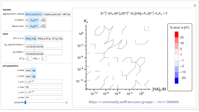
Contour plot of error in calculation of [+H]
Contour plot of error in calculation of ]
[
+
H
This program illustrates the percent error of the calculated solution for ] using each approximation equation. The contour plot of two selected variables shows regions of error ranges from no error (white) to highly positive (red) and highly negative (blue).
[
+
H
To generate the plot, the approximation equation (approximation method, numerator, denominator) is selected. Two out of three variables (, , ) are selected as the x and y values for the plot. The third variable z = ax + b can be set to vary with x or as a constant. values for the approximation and the exact calculation can be input separately. In addition, the two axes can be set to be in linear (none) or log scale and the minimum and maximum values of the axes can be adjusted. The number of plot points (initial sample points) can be adjusted to obtain smoother or rougher plots. Increasing the number of plot points increases the smoothness of the plot along with the evaluation time.
[HA]
0
[]
-
A
0
K
a
K
w
In[]:=
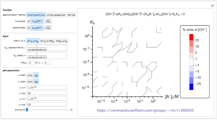
Contour plot of error in calculation of [-OH]
Contour plot of error in calculation of ]
[
-
OH
This program illustrates the percent error of the calculated solution for ] using each approximation equation. The contour plot of two selected variables shows regions of error ranges from no error (white) to highly positive (red) and highly negative (blue).
[
-
OH
To generate the plot, the approximation equation (approximation method, numerator, denominator) is selected. Two out of three variables (,, ) are selected as the x and y values for the plot. The third variable z = ax + b can be set to vary with x or as a constant. values for the approximation and the exact calculation can be input separately. In addition, the two axes can be set to be in linear (none) or log scale and the minimum and maximum values of the axes can be adjusted. The number of plot points (initial sample points) can be adjusted to obtain smoother or rougher plots. Increasing the number of plot points increases the smoothness of the plot along with the evaluation time.
[]
-
A
0
[HA]
0
K
b
K
w
In[]:=
CITE THIS NOTEBOOK
CITE THIS NOTEBOOK
Approximation of pH and associated error in monoprotic acid and base solutions
by Weerapat Chiranon, Sopanant Datta, Junming Ho and Taweetham Limpanuparb (in alphabetical order)
Wolfram Community, STAFF PICKS, September 7, 2023
https://community.wolfram.com/groups/-/m/t/3008305
by Weerapat Chiranon, Sopanant Datta, Junming Ho and Taweetham Limpanuparb (in alphabetical order)
Wolfram Community, STAFF PICKS, September 7, 2023
https://community.wolfram.com/groups/-/m/t/3008305