This paper presents a computational analysis of force and kinematics revolving around a prosthetic hand model. Founded on grasp map calculations, along with forward and inverse kinematic modeling, we extend our exploration of prosthetics’ functioning mechanism and their implications for amputee patients in daily life. With principles from linear algebra and mechanical physics, we derive the minimum 3D force required to balance an object against gravity. Forward kinematics is used to guide the hand in grasping an object while adhering to joint constraints and structural limitations. Our approach to inverse kinematics and joint movement introduces a novel algorithm for identifying the intersection region between the hand and the object. We ultimately analyze the force distribution across specific contact positions using grasp map simulations, applying our model to balance a range of objects, from simple dimensions to randomly generated polyhedrons.
Introduction
Introduction
Ethiopia,home to about 126 million people and the second-most-populous nation in Africa, experiences impoverished, underserved public healthcare issues; among the most is limb loss. Recent systematic reviews reveal a striking 31.7% pool of the population having a limb amputation, with lower-limb procedures twice as prevalent as upper-limb cases (Sume). Despite the absence of precise number of amputees, field studies suggest that amputations are one of the most least-documented, particularly in rural regions where injury surveillance is limited and adequate healthcare is scarce. Recently, the increased conflicts in the northern Tigray way left thousands with permanent disabilities, exceeding 43,000 former combatants requiring long-term care due to the limb loss (Getachew, 2025).
Conventional prosthetic-hand models are generally exorbitant, being merely used for cosmetic purposes. Hence, we explore the Body powered prosthetics, which uses motions of the body to activate the hand: most common involve pulling a cable when the arm is moving forward for the flexion control, or utilizing upper arm joints. Thus, it is critical to optimize the usage of these prosthetic hands in daily life, from grabbing a cup to manipulating various 3D objects by building a grasp manipulation task.
Conventional prosthetic-hand models are generally exorbitant, being merely used for cosmetic purposes. Hence, we explore the Body powered prosthetics, which uses motions of the body to activate the hand: most common involve pulling a cable when the arm is moving forward for the flexion control, or utilizing upper arm joints. Thus, it is critical to optimize the usage of these prosthetic hands in daily life, from grabbing a cup to manipulating various 3D objects by building a grasp manipulation task.
Prosthetic Hand Model
Prosthetic Hand Model
Mesh Files Initialization
Mesh Files Initialization
The finger and palm shells used for the prosthetic throughout this study are taken from the e-NABLE’s Raptor 2 body-powered hand model. e-NABLE is a global volunteer network that manufactures freely modifiable 3D-printed limb components, providing a “helping hand” to communities.
A human hand is composed of three rigid links: proximal phalanx, middle/distal phalanx, and fingertip. With total of 14 finger parts (considering the thumb has only two), we have condensed down each finger into its segments and directly deploying the STL mesh files on the notebook for easy access and 3D visualization.
Fingers STL
Fingers STL
In[]:=
(*Finger 1: Index Finger*)proximal1= ;distal1=
 ;tip1 =
 ;(*Finger 2: Middle Finger*)proximal2=
 ;distal2=
 ;tip2=
 ;(*Finger 3: Ring Finger*)proximal3 =
 ;distal3=
 ;tip3 =
  ;(*Finger 4: Pinky Finger*)proximal4=
 ;distal4=
 ;tip4=
 ;(* Finger 5: Thumb *)distal5=
 ;tip5=
 ;
;
Palm STL
Palm STL
In[]:=
palm= ;
;
Building the Hand
Building the Hand
After fetching the data for the hand STL files, we import and visualize the finger segments on a 3D space. However, the finger parts have their respective position and orientation, meaning that we have to rotate and translate the object to form a hand model. We constructed functions that operates this task:
In[]:=
proximalFindInitialPosition[stl_,translate_]:=Translate[Rotate[Rotate[stl,Pi/2,{0,0,-1},{0,0,0}],Pi/2,{0,1,0}],translate];proximal1=proximalFindInitialPosition[proximal1,{-5,1.5,-28}];proximal2=proximalFindInitialPosition[proximal2,{-8.5,3.5,-25}];proximal3=proximalFindInitialPosition[proximal3,{-14,5,-24.4}];proximal4=proximalFindInitialPosition[proximal4,{46,-92.5,-25}];
The function above re-adjusts the orientation of the proximal phalanx segments for each finger.
In[]:=
distalFindInitialPosition[stl_,translate_]:=Translate[Rotate[Rotate[stl,Pi/2,{0,0,-1},{0,1,0}],Pi/2,{0,1,0}],translate];distal1=distalFindInitialPosition[distal1,{0,1.5,0}];distal2=distalFindInitialPosition[distal2,{-2,3.5,4.5}];distal3=distalFindInitialPosition[distal3,{-7,4.5,4}];distal4=distalFindInitialPosition[distal4,{-8,8,6}];distal5=Rotate[Translate[Rotate[distal5,Pi,{1,0.5,0.3},{0,0,0}],{-14,43,-35}],Pi/10,{1,0,0}];
Same implementation is applied for the middle/distal phalanx segments.
In[]:=
tipFindInitialPosition[stl_,translate_]:=Translate[Rotate[Rotate[stl,Pi/2,{0,1,0}],Pi/2,{-1,0,0}],translate];tip1=tipFindInitialPosition[tip1,{0,1.8,25}];tip2=tipFindInitialPosition[tip2,{-2,3.5,30}];tip3=tipFindInitialPosition[tip3,{-7,4,29}];tip4=tipFindInitialPosition[tip4,{-6,7,30}];tip5=Rotate[Translate[Rotate[tip5,Pi,{1,0.5,0.3},{0,0,0}],{-51,84,-78}],Pi/10,{1,0,0}];
The finger tips has been displaced and rotated for mapping the hand model in a 3D dimension.
In[]:=
palm=Translate[Rotate[Rotate[palm,Pi/2,{0,-1,0}],Pi,{0,1,40}],{-110,0,-20}];
And lastly, the palm undergoes the transformation. Although there are other options, such as RotationTransform or TranslationTransform, for the identical task, we have manually adjusted their orientation for precisely visualizing the hand. Hence, finding the 3D-coordinates for transformation was challenging.
Simulating Joint Movements
Simulating Joint Movements
Joint Movements
Joint Movements
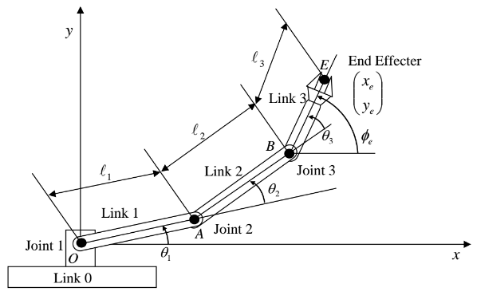
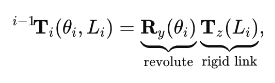
Each finger is modelled as a planar 3-R serial chain where the three revolving joints in the fingers have a parallel rotation axes and are co-linear with the anatomical y-axis. Here, θ1 represents the angle between the proximal phalanx and the palm, θ2 for the angle between the proximal phalanx and the distal phalanx, and θ3 for the distal phalanx and the fingertip.
Let,
Let,

(
1
)Here, the variable s changes the angle between the finger segments over time, animation their movements.
Although we will be discussing about Forward Kinematics later in the study, this is an abstract representation of the movements for the finger parts.
(
2
)
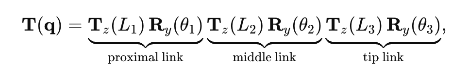
With L1, L2, and L3 representing the respective length of the finger parts, we calculate the translation and rotation required to move the fingers together while joined in a chain. We have applied the same principle in the following code:
With L1, L2, and L3 representing the respective length of the finger parts, we calculate the translation and rotation required to move the fingers together while joined in a chain. We have applied the same principle in the following code:
Finger Movement Graphics for the Index, Middle, Ring, and Pinky Finger
In[]:=
ClearAll[fingerGraphics,thumbGraphics]fingerGraphics[L1_,L2_,L3_,base_,prox_,dist_,tip_,s_,pivot1_,pivot2_,pivot3_]:=Module[{θ1,θ2,θ3,seg1End,seg2End},θ1=(Pi/2)s;θ2=0.75θ1;θ3=0.7θ2;seg1End=base+{L1Cos[θ1],0,-L1Sin[θ1]};seg2End=seg1End+{L2Cos[θ1+θ2],0,-L2Sin[θ1+θ2]};{Translate[Rotate[prox,θ1,{0,1,0},pivot1],base],Translate[Rotate[dist,θ1+θ2,{0,1,0},pivot2],seg1End],Translate[Rotate[tip,θ1+θ2+θ3,{0,1,0},pivot3],seg2End]}]
The function fingerGraphics employs the forward kinematics for the segments with the rotation axis centered at the y-axis. The seg1End and seg2End both display the end points of each finger parts, demonstrating the joint movement within a finger.
The function fingerGraphics employs the forward kinematics for the segments with the rotation axis centered at the y-axis. The seg1End and seg2End both display the end points of each finger parts, demonstrating the joint movement within a finger.
Finger Movement Graphics for the Thumb
In[]:=
thumbGraphics[base_,dist_,tip_,s_]:=Module[{θ1,θ2,seg1End},θ1=(Pi/2)s;θ2=0.75θ1;seg1End=base+{10Cos[-θ1],0,-10Sin[-θ1]};{Translate[Rotate[dist,-θ1,{1,1,2},{-55,40,-50}],base],Translate[Rotate[tip,-(Abs[θ1]+θ2),{1,1,3},{-45,45,-50}],seg1End]}]
As shown in thumbGraphics, the thumb is only composed of 2 rigid phalanges with different axis of rotation compared to others. Based on these implementation, we are able to visualize the hand prosthetic in Wolfram, with each finger joints and segments moving while being aligned to one another.
As shown in thumbGraphics, the thumb is only composed of 2 rigid phalanges with different axis of rotation compared to others. Based on these implementation, we are able to visualize the hand prosthetic in Wolfram, with each finger joints and segments moving while being aligned to one another.
Combined Manipulate Animation
Combined Manipulate Animation
Animation for the Finger Joint Movements
In[]:=
Manipulate[Graphics3D[Join[(*Palm*){palm},(*IndexFinger*)fingerGraphics[35,25,30,{0,0,0},proximal1,distal1,tip1,s,{0,0,0},{0,0,0},{0,0,0}],(*MiddleFinger*)fingerGraphics[35,25,30,{0,0,0},proximal2,distal2,tip2,s,{0,0,0},{0,0,0},{0,0,0}],(*RingFinger*)fingerGraphics[33,25,30,{0,0,0},proximal3,distal3,tip3,s,{-10,0,0},{-10,0,0},{-10,0,0}],(*PinkyFinger*)fingerGraphics[16,15.5,30,{0,0,0},proximal4,distal4,tip4,s,{-20,0,0},{-15,0,0},{-14,2,-2.5}],(*Thumb*)thumbGraphics[{0,0,0},distal5,tip5,s]],Boxed->False,Axes->False,AxesLabel->{"x","y","z"},PlotRange->All,ImageSize->Large,ViewPoint->{1,0,-1.5}],{{s,0.,"Fold"},0.,0.8,ControlType->Animator,AppearanceElements->"ProgressSlider",AnimationRunning->False,AnimationRepetitions->1},TrackedSymbols:>{s},SaveDefinitions->True]
Out[]=


Kinematics
Kinematics
Forward Kinematics
Forward Kinematics
As introduced before in 2.3, Forward Kinematics determines the position and orientation of the end-point of the tip, so-called as the end-effector, based on the values for the joint and length variables, including the angles between the links in the vase of revolution or rotation. (Citation). Albeit commonly used in robotics, a finger is composed of a set of links connected together by joints in between just like a robot arm. Specifically to the fingers, a Metacarpophalangeal (MCP) joint connects the finger bones (phalanges) to the bones of the palm (metacarpals). Also, acknowledge that a revolute joint acts as a hinge, which is the primarily joint used for the finger movements.
Link Transformation
Link Transformation
The following values were used to calculate the position and orientation of the finger segments . The multiplier before the angles are incorporated to reflect the tendon cam in e - NABLE prosthetic hands . The first joint MCP pulls the cable the most, while the DIP pulls the least.
The following values were used to calculate the position and orientation of the finger segments . The multiplier before the angles are incorporated to reflect the tendon cam in e - NABLE prosthetic hands . The first joint MCP pulls the cable the most, while the DIP pulls the least.
Lengths
In[]:=
{L1,L2,L3} = {35.,25.,30.};
Angles
In[]:=
θ1 = (Pi/2)finger1Fold;θ2 = 0.75 θ1;θ3 = 0.70 θ2;
Based on the specifications of the lengths and angle, we are able to calculate the end points of each joints for the finger.
End Points
In[]:=
base + {L1 Cos[θ1],0,-L1 Sin[θ1]};seg2End = seg1End + {L2 Cos[θ1+θ2],0,-L2 Sin[θ1+θ2]};
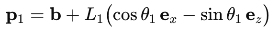

The negative value of z component indicates that the movement of the fingers move down, producing -Sinθ as a result. The Cosine component provides the adjacent figure, the x-projection while the Sine component provides the z-projection in the frame. The cumulative angle is grounded from the fact that θ2 is rotating in respect to θ1, which is derived by the sum of the two joint angles.
End-Effector
In[]:=
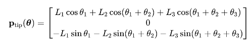
seg3End = seg2End + {L3 Cos[θ1+θ2+θ3],0,-L3 Sin[θ1+θ2+θ3]};
As a result, we are about to find the position of the finger-tip, which is the End-Effector.
In[]:=
Out[]=
Based on the position of the joints, we are able to transform the finger segments in regards to them.
Rotation & Transformation
In[]:=
g1 = Translate[Rotate[proximal1,θ1,{0,1,0}],base];g2 = Translate[Rotate[distal1,θ1+θ2,{0,1,0}],seg1End];g3 = Translate[Rotate[tip1,θ1+θ2+θ3,{0,1,0}],seg2End];
Below is an animation that visualizes the translation and rotation of the finger segments (If the segments look off try moving the slider bar!)
Full Code for Animation
Full Code for Animation
Manipulate[Module[{base={0,0,0},L1=35.,L2=25.,L3=30.,θ1,θ2,θ3,seg1End,seg2End,seg3End,g1,g2,g3},θ1=(Pi/2)finger1Fold;θ2=0.75θ1;θ3=0.70θ2;seg1End=base+{L1Cos[θ1],0,-L1Sin[θ1]};seg2End=seg1End+{L2Cos[θ1+θ2],0,-L2Sin[θ1+θ2]};seg3End=seg2End+{L3Cos[θ1+θ2+θ3],0,-L3Sin[θ1+θ2+θ3]};g1=Translate[Rotate[proximal1,θ1,{0,1,0}],base];g2=Translate[Rotate[distal1,θ1+θ2,{0,1,0}],seg1End];g3=Translate[Rotate[tip1,θ1+θ2+θ3,{0,1,0}],seg2End];Graphics3D[{g1,g2,g3},Boxed->True,Axes->True,AxesLabel->{"x","y","z"},PlotRange->All,ImageSize->Medium,ViewPoint->{1,-1,1}]],{{finger1Fold,0.,"Index finger flexion"},0,1.3},AppearanceElements->{"OpenCloseButton","ResetButton"},SaveDefinitions->True]
Inverse Kinematics
Inverse Kinematics
Inverse Kinematics is the “backward” process of Forward Kinematics, which essentially computes the position and angle of the joints of each robotics arms (finger segments in this case) needed to achieve a desired position of the End-Effector. In simple terms, it is the process of manipulating the finger segments to move it to the desired point while forward kinematics calculates the endpoint based on the joint angles and orientation. There are various Inverse Kinematics algorithms that exist, including the Jacobian Inverse Kinematics, Joint-limit Enforcement, and FABRIK (FAst BI-directional Reaching Inverse Kinematics), which we will be implementing for this study. FABRIK is effective for hand movements since the joints are challenging to express in a trigonometric dimension.
FABRIK Framework
FABRIK Framework
Angle Calculator
This is a helper function to determine the angle between Vector 1 and Vector 2, which is expressed based on two consecutive joints . The objective of the function is to calculate the vector angle between the two joints and limit it to the finger constraints . Generally, from 0 to 90 - 100 degrees of rotation is accepted for the joint movements . FABRIK is founded on iterative procedures to configure the position of the joints to reach the endpoint while moving under constraints.
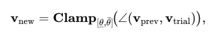
As shown in the formula, the new vector will Clamp the current vector to be confined within the mechanical range. This occurs when the current angle vector is bigger or smaller than the bounds.
Code Implementation of Finding the Angle
In[]:=
findAngle[p1_, p2_, bounds_] := Module[{theta1, theta2, deltaθ, boundVector, assoc}, (*Considering both Cases: Angle / 2*PI - Angle*) theta1 = VectorAngle[p1, p2]; theta2 = 2 Pi - theta1; (*If the angle is Off-bounds, it will calculate the closest bound vector*) If[bounds[[1]] <= theta1 <= bounds[[2]] || bounds[[1]] <= theta2 <= bounds[[2]], p2, boundVector = { RotationMatrix[bounds[[1]], Cross[p1, p2]] . p1, RotationMatrix[bounds[[2]], Cross[p1, p2]] . p1, RotationMatrix[2 Pi - bounds[[1]], Cross[p1, p2]] . p1, RotationMatrix[2 Pi - bounds[[2]], Cross[p1, p2]] . p1}; (*It will "snap" the position vector to the closest bound*) boundVector = N@Normalize[#]*Norm[p2] & /@ boundVector; deltaθ = VectorAngle[p2, #] & /@ boundVector; AssociationThread[deltaθ, boundVector][Min@deltaθ] ] ]
In[]:=
1
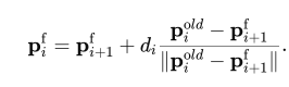
.Forward Reach: In this stage, we assume the finger-tip snaps to the end point ‘target’. From the back, the joints moves towards the target while maintaining the length between the two joints, fixing them to a new position. The position should be within the mechanical bound and if it exceeds the limit, the algorithm will the closest bound vector. Mathematically, we express this as:
In code implementation, it would look as the following:
In[]:=
forwardReach[pos_, lengths_, target_, angleConst_, maxVector_] := Module[{p = pos, dist, vec, vec1, vec2, newVec, oldVector, newVector, aVec}, p[[-1]] = target; Table[dist = EuclideanDistance[p[[x + 1]], p[[x]]]; vec = p[[x]] - p[[x + 1]]; p[[x]] = p[[x + 1]] + vec*lengths[[x]]/dist; If[x < Length[p] - 1, vec2 = p[[x]] - p[[x + 1]]; vec1 = p[[x + 2]] - p[[x + 1]]; newVec = findAngle[vec1, vec2, angleConst[[x]]]; p[[x]] = p[[x + 1]] + newVec]; oldVector = pos[[x]] - pos[[x + 1]]; newVector = p[[x]] - pos[[x + 1]]; aVec = findAngle[oldVector, newVector, {-maxVector, maxVector}]; p[[x]] = pos[[x + 1]] + aVec, {x, Length[p] - 1, 1, -1}]; p]
2
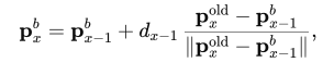
.Backward Reach: After the Forward Reach, the algorithm must bring the finger back to its original anchor while maintaining the finger lengths and mechanical bounds. We use the same iterative approach in 1. to move the joint positions while calling the fingAngle function to confine the angle within its bounds. From x to x+1 looping, the iteration now goes backwards from x to x-1.
In[]:=
backwardReach[pos_, lengths_, base_, angleConst_, maxVector_] := Module[{p = pos, dist, vec, vec1, vec2, newVec, oldVector, newVector, aVec}, p[[1]] = base; Table[dist = EuclideanDistance[p[[x]], p[[x - 1]]]; vec = p[[x]] - p[[x - 1]]; p[[x]] = p[[x - 1]] + vec*lengths[[x - 1]]/dist; If[x > 2, vec2 = p[[x]] - p[[x - 1]]; vec1 = p[[x - 2]] - p[[x - 1]]; newVec = findAngle[vec1, vec2, angleConst[[x - 2]]]; p[[x]] = p[[x - 1]] + newVec]; oldVector = pos[[x]] - pos[[x - 1]]; newVector = p[[x]] - pos[[x - 1]]; aVec = findAngle[oldVector, newVector, {-maxVector, maxVector}]; p[[x]] = pos[[x - 1]] + aVec, {x, 2, Length[p]}]; p]
3
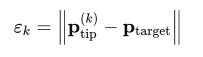
.Iterate 1. and 2. until the positional error is less than the threshold, meaning the distance between the finger-tip and the endpoint is down to the tolerance level (usually 1 mm), allowing the prosthetic fingers to reach a targeted point in a 3D plane.
In[]:=
fabrikStep[pos_,lengths_,target_,angleConst_,maxVector_]:=Module[{p1,p2},p1 = forwardReach[pos,lengths,target,angleConst, maxVector];p2 = backwardReach[p1,lengths,pos[[1]],angleConst,maxVector];<|"Positions"->p2,"Error"->EuclideanDistance[p2[[-1]],target]|>];
Out[]=

Running the Full Code
Running the Full Code
Random Polyhedrons
Random Polyhedrons
Having established both the Forward Kinematics and Inverse Kinematics, we now explore their practical application in the real world, especially when interacting objects. We focus on randomly generated polyhedra, identifying every potential contact point and calculate the corresponding contact force by the prosthetic hand. A prerequisite is an algorithm for extracting outward-facing normal vectors from any polyhedron. While Wolfram’s ResourceFunction[“PolyNormalVector”] offers this function, it provides little detail on computing a normal for an arbitrary face of an arbitrary mesh. We therefore present a method for deriving face normals directly from the vertex and face lists of any polygonal object in Wolfram.
Initial Setup / Mesh Polyhedrons
Initial Setup / Mesh Polyhedrons
We first choose a random polyhedron, discretizing the region and meshing the boundary for further manipulation.
In[]:=
reg = Scale[BoundaryMesh[DiscretizeRegion[RandomPolyhedron[]]], {2, 2, 2}];
The object is split into its respective coordinates and polygons that construct the shape.
In[]:=
Polys=MeshCells[reg,2];Coord=MeshCoordinates[reg];centerOfMass=RegionCentroid[reg];
The first line bundles shared vertices and indexed faces into a compact GraphicsComplex and expands that object so each face is listed with full coordinate triples.
In[]:=
body=GraphicsComplex[Coord,Polys];faces=Normal[GraphicsComplex[Coord,Polys]];
In[]:=
Graphics3D[Join[{reg},{Purple,Point[#]&/@Coord}],Lighting->"Accent",Boxed->False,ImageSize->Large];
In[]:=


For visualization purposes, we choose random faces and finds the corresponding polygons and the centroid in the polygons.
In[]:=
listPoly = Table[Polygon[faces[[RandomInteger[Length[faces]]]][[1]]],5]; centroid = Table[Mean[listPoly[[x]][[1]]],{x,5}]; normal = Chop[Table[ResourceFunction["PolygonNormalVector"][listPoly[[i]]],{i,5}],10^-10];
We find the normal vector of those polygons, which will be visualized as an arrow from the centroid of the polygons.


Grasping a Polyhedron
Grasping a Polyhedron
Initialization
Initialization
In[]:=
ClearAll["Global`*"];
Function Polyhedron generates a random polyhedron of its number of points and faces. We use this property to find the coordinates and faces in a polyhedron where the fingers contact with.
In[]:=
RandomPolyhedron[]
Out[]=
Polyhedron
We apply the same principal mentioned in 3.3
In[]:=
reg=Scale[BoundaryMesh[DiscretizeRegion[RandomPolyhedron[]]],2];
In[]:=
poly=Translate[Scale[reg,{3,2,2}],{-0.5,-1.5,-2}]
Out[]=

WCK Algorithm: Find Contact Points with Polyhedron
WCK Algorithm: Find Contact Points with Polyhedron
Established by William Choi-Kim (& Aayush Dubey), this algorithm operates as an alternative approach to Forward and Inverse kinematics. One of the challenges in implementing kinematics in hands is that most finger segments rotate in a certain trajectory, hence, computing every subsequent joint’s position would seem improbable. The ADWCK framework optimizes the contact point with a polyhedron, searching the 3 respective joint angles for each finger to reach that point. It changes the angle for each finger segments to rotate until the finger tip, or End-effector, intersects with the surface of the polyhedron.
fingers[fb1_ (*first joint*), fb2_ (*second and third joint*), shape_] := Module[{ roots = { (*index*){0, 0, 0},(*middle*){-1, 0, 0},(*ring*){-2, 0, 0},(*pinky*){-3, 0, 0},(*thumb*) {1, -0.5, 0} }, fingerPos, fingerEnds, fingerIntersects, coord = MeshCoordinates[shape], polys = MeshCells[shape, 2], body, faces, isIntersecting, onlyEndJointInRegion }, (*Random Polyhedron*) body = GraphicsComplex[coord, polys]; faces = Normal[GraphicsComplex[coord, polys]]; (*Moves the finger joints to certain angle*) fingerPos = Join[ AnglePath3D[roots[[#]], {{0, {Pi/2, 0, 0}}, {2, {0, fb1[[#]], 0}}, {2, {0, fb2[[#]], 0}}, {2, {0, fb2[[#]], 0}}}] & /@ Range[4], { AnglePath3D[roots[[5]], {{0, {0, 0, 0}}, {3, {0, fb1[[5]], 0}}, {2, {0, fb2[[5]], 0}} }] } ]; fingerEnds = #[[-2 ;; -1]] & /@ fingerPos; (*Checks if the finger intersects with the polyhedron*) fingerIntersects = Table[RegionIntersection[Line[end], #] & /@ faces, {end, fingerEnds}]; fingerIntersects = Table[Select[Thread[finger -> Range[Length[finger]]], ToString[Head[#[[1]]]] == "Point" && Length[#[[1]]] == 1 &], {finger, fingerIntersects}]; (*Search for all points of intersection*) onlyEndJointInRegion = And @@ Table[! RegionMember[shape, joint], {joint, #[[;; -2]]}] & /@ fingerPos; (*If intersecting, returns the point and corresponding faces*) isIntersecting = Table[ If[Length[fingerIntersects[[finger]]] > 0 && onlyEndJointInRegion[[finger]], (*has intersection*) {fingerIntersects[[finger]][[1]][[1]], faces[[fingerIntersects[[finger]][[1]][[2]]]]}, Missing["The finger does not intersect"] ] , {finger, Length[roots]}]; {And @@ (! MissingQ[#] &) /@ isIntersecting, isIntersecting, fingerPos} ];
This algorithm evaluates if the finger is intersecting the polyhedron and lists all the successful cases; extended overlaps such as edge glances or embedded lines are ignored. From a long list of “Missing”, there will be records where a point is intersected, which the program will print out along with its corresponding face indices in the body. This allows us to compute the force required to balance the object when contacting the points and their corresponding faces. Our algorithm takes into account for cases where the finger does not intersect the object due to its size and dimension, thus, will print out the number of contact points for the fingers which are plausible. An example computation of this code would display the following:
1-8.75436×,-1.4297,-2.38491,2{-1.,-1.12764,-1.8349},5{-0.398924,-0.5,-2.45181},1Polygon,2Polygon,5Polygon
-17
10
This animation is not generated via code; however, it is the ultimate result for the fingers[] function: finding the contact points
This animation is not generated via code; however, it is the ultimate result for the fingers[] function: finding the contact points

Compute the Angle
Compute the Angle
The angleCombinationPossibilities[] function finds the angle for each segments for the five fingers. The function goes through a iteration of possible angle combinations possible for flexion, particularly one that produces a first-touch with the polyhedron. Starting from the finger being straight, the routine sweeps θ₁ from 0 to 90 degrees (π /2 rad) based on incremental steps. For every combination, it will validate the pose by
◼
(i) Confirm that the fingertip’s segment intersects at least one mesh face
◼
(ii) Ensure all proximal joints remain outside the solid, thereby ensuring the fingertip is the first part of contact
As soon as a pair of angles satisfy these criteria, the successful angles are recorded; trials that never achieve contact are discarded. The final product will be a five lists of acceptable angle pair {θ1, θ2}, one per finger. The initial stepSize of 0.02 will take around 20 minutes or more, in worse scenarios, the program may crash. For such instances, deduce the stepSize to 0.1 or 0.2 which requires less computation and time.
poly;angleCombinationPossibilities = Table[ Module[{fingerAng = {0, 0, 0, 0, 0}, working, everyPossibility, stepSize = 0.05, a2}, everyPossibility = ParallelTable[ (*Combination of θ1 and θ2*) fingerAng = {{0, 0, 0, 0, 0}, {0, 0, 0, 0, 0}}; working = False; a2 = 0; While[ ! working && a2 <= 2 Pi/3, fingerAng[[1]][[ind]] = a1; fingerAng[[2]][[ind]] = a2; (*running the fingers[] function to validate i*) working = ! MissingQ[fingers[fingerAng[[1]], fingerAng[[2]], poly][[2]][[ind]]]; If[working, Nothing, a2 += stepSize]; ]; If[working, {a1, a2}, False], {a1, 0, Pi/2, stepSize}]; Select[everyPossibility, Length[#] > 0 &] ], {ind, 5}]
Example Angle Combination
Example Angle Combination
Grasp-Map Manipulation
Grasp-Map Manipulation
Grasp Maps
Grasp Maps
In robotics, we break the study of multi-fingered hands to two sections: kinematics and planning, and dynamics and control. As we have explored the kinematics part of multi fingered hands, we now examine the force mechanism regarding the object. Through this, we attempt to find the relationship between forces and motions of the interacting objects and fingers. As we have the points and surfaces of contact given, we are able to compute the fundamental grasping map, calculating the contact forces needed for force equilibrium.
The grasp mapping grants the ability to resist external forces. With an external wrench applied to the object, which the study focuses on gravity, we generate an opposing wrench to this force, imposed on the contact points for a force-closure grasp.
The grasp mapping grants the ability to resist external forces. With an external wrench applied to the object, which the study focuses on gravity, we generate an opposing wrench to this force, imposed on the contact points for a force-closure grasp.
Initialization
Initialization
For this study, we will be using the parameters obtained by the training above to determine whether the grasp map functions. In later versions, we will examine how different polyhedrons and different points can alter the results and force equilibrium.
In[]:=
poly =  ;points = {{4.0706363164855017`*^-17,0.6647853600433429`,-2.8827912092221095`},{-1.`,0.2180692744922566`,-3.1173463090142772`},{-1.9999999999999998`,0.7830429674765944`,-3.185971107297219`}};polygs = Polygon,Polygon,Polygon;pRef=RegionCentroid[poly];normal=Table[ResourceFunction["PolygonNormalVector"][polygs[[i]]],{i,3}];normals=-normal;
Tangential Pair [Force + Torque]
Tangential Pair [Force + Torque]
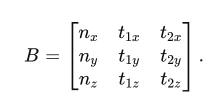
For every finger contact, we must consider the 3-dimensional force and torque acting upon the surface. This includes the surface normal n̂ (pushing direction, not pulling).To express the frictional force that opposes gravity, we need two perpendicular tangent directions towards the surface of the polyhedron. Together, we get the following matrix:
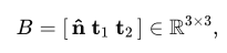
This matrix will be [3x3] taking into account the x, y, z component of the force vectors pushing the object surface. In order to compute the accurate tangent vectors, we first obtain the first tangent in regards to the fixed world axis. If n̂ is not parallel to the global z-axis, we use the z-component {0 , 0 , 1} as well. Else, we assign {0 , 1 , 0} to avoid the product becoming a 0. This will result in the orthonormal dimensions for any surface orientation even when the contact normal points near Z.
In[]:=
ClearAll[tangentPair];tangentPair[n_]:= Module[{t1}, t1=Normalize[Cross[normals[[n]], If[Abs[normals[[n]].{0,0,1}]<0.9,{0,0,1},{0,1,0}]]]; {t1,Cross[normals[[n]],t1]}];tangent = Join[Table[tangentPair[x],{x,3}]];
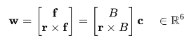
Next it constructs, for that same contact point, a [6 x 3] matrix whose top three rows are the force basis
and whose bottom three rows are the corresponding torque directions obtained by crossing each basis vector with the moment arm.
and whose bottom three rows are the corresponding torque directions obtained by crossing each basis vector with the moment arm.
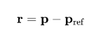
Multiplying the torque matrix with the three force components, yields the full six - dimensional wrench that the single contact can apply to the object .
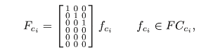
In[]:=
ClearAll[contactBlock];contactBlock[p_,nHat_,{t1_,t2_}]:= Module[{r=p-pRef}, With[{B=Transpose[{nHat,t1,t2}]},ArrayFlatten[{{B},{Cross[r,#]&/@B}}]]];
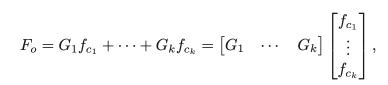
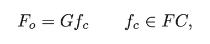
Assembling these [6 x 3] contact blocks for all fingertips later produces the global grasp matrix G.
Since we have 3 fingers that are having contact with the polyhedron we will be using a [6 x 9] Matrix to represent grasp maps.
Since we have 3 fingers that are having contact with the polyhedron we will be using a [6 x 9] Matrix to represent grasp maps.
Grasp Maps [6 x 3(Number of Contact Finger)]
Grasp Maps [6 x 3(Number of Contact Finger)]
Gblocks = MapThread[contactBlock, {points, normals, tangent}, 1];Transpose@Partition[Flatten@Gblocks,6]//MatrixForm
Out[]//MatrixForm=
-0.212987 | 0.976396 | -1.66814 | -0.212987 | 0.976396 | -1.22171 | 0.235681 | -0.438056 | 0.363078 |
-0.977025 | -0.213124 | 0.219979 | -0.977025 | -0.213124 | -0.770959 | -0.96502 | 0. | 2.06943 |
0.00764876 | -0.0350643 | 0.0599061 | 0.00764876 | -0.0350643 | 0.043874 | -0.114847 | -0.898948 | 2.02852 |
-0.0358888 | -1.15389 | -0.313019 | -0.0358888 | -1.38647 | -0.347344 | -0.867503 | -1.65018 | -1.60684 |
0. | 0.252969 | -1.15969 | 0. | 0.310575 | -1.42377 | -0.262175 | -0.562218 | -0.982678 |
-0.999356 | 0.182354 | -1.66759 | -0.999356 | 1.06423 | -1.01829 | 0.422733 | 1.33773 | 0.783013 |
In[]:=
mass = RegionMeasure[reg];externalWrench = {{0}, {0}, {mass * (9.8)}, {0}, {0}, {0}};
We take the gravity as the external wrench acting upon the object, assuming the object’s density is 1. We will hence take the volume of the polyhedron and multiply with g, approximately of 9.81 . This provides us with a wrench matrix of [6 x 1], which will be multiplied with the grasp map G onwards.
-2
ms
In[]:=
Dimensions /@ {Gblocks, externalWrench};wext = Flatten[externalWrench];G = ArrayFlatten[{Gblocks}];vars = Array[c, 3*3];
In order to find the total contact force of the fingers that equal out the gravity, we need to have 3n size of contact forces (accounting of x, y, z), which in case will be a [9 x 1] as we have 3 contact points.
In[]:=
Fundamental Grasping Constraint
Fundamental Grasping Constraint
Force Closure - The ability to resist external forces
Force Closure - The ability to resist external forces
To verify that a given set of contact points affords force closure—that is, the ability to generate internal contact forces that exactly cancel any external wrench
In[]:=
μ=0.6;vars=Array[c,9];
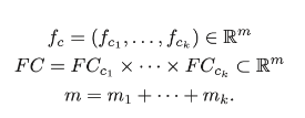
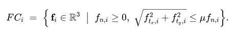
Based on the aforementioned information, we have to set constraints that would give us the contact forces that are required to balance the weight. For each contact i, the linearized Coulomb cone in 3-space: a non-negative normal component and a circular bound of slope μ for the tangential pair. These inequalities guarantee that every candidate vector lies inside the physically admissible contact set
In[]:=
coneCons=Table[{vars[[3 i]]>=0,Norm[vars[[{3 i-2,3 i-1}]]]<=μ vars[[3 i]]},{i,3}];wrenchCons=Thread[G.vars+wext==0];allCons=Join[Flatten[coneCons],wrenchCons];sol=NMinimize[{vars.vars,allCons},vars];Array[c,3*3]/. sol[[2]];
Based on this output we are able to deduce that there are no contact forces that satisfy the conditions for a grasp map, which is confirmed by this code below.
In[]:=
If[NumericQ[sol[[1]]],sol[[2]],Print["There are no points that satisfy the constraints "]]
There are no points that satisfy the constraints
Optimization of the Contact Points
Optimization of the Contact Points
Future Works
Future Works
This project could be extended in multiple ways:
◼
Using the FABRIK inverse kinematics described in Section 3.2 to animate the hand mesh’s movement toward the object, grasping it at points that would actually satisfy the constraints described in Section 4. Currently, the hand’s movement is governed by a forward kinematic system that moves the hand until a tolerance is reached. FABRIK would provide much more accurate grasping dynamics and more satisfactory results.
◼
There are several types of contacts that could’ve been used as the wrench basis. The one we focused on was a hard-point finger with friction. This would require each finger to have its own wrench basis, but it would be interesting to observe the effects and analyze their forces differently than was in the more simple implementation considered here.
◼
My simulation was to see if we can satisfy the force-closure grasp constraint given a set of points. The next step would be to make an attempt to satisfy the second constraint, namely if the grasp is manipulable. Then we can test it out by moving it to a random location, again using the FABRIK inverse kinematics algorithm implemented earlier.
◼
Dex-Net is a popular grasping NN - It would be a good extension to use a prosthetic hand like this to repeatedly simulate a bunch of hand orientations and finger fold combinations, so that we can pass it to the neural net to determine what sort of grasping constraints can yield a force-closure grasp. This would provide an even better solution to the problem of optimal grasp.
Conclusion
Conclusion
Overall, we were able to demonstrate kinematics and grasp maps demonstration in Wolfram based on our hand prosthetic model from e-NABLE. We have built the kinematic model, detecting fingertip contacts using WCK algorithm, and eventually computing the contact force needed to balance the weight wrench. We have tested the contact force using grasp maps with complex matrices. Although we were not able to compute the forces, we are able to find the forces and friction cones through iterative, repetitive computation in the future. In future work, we will further expand our implications of kinematics and grasp maps when designing for 3D printed prosthetic models, as well as expanding the project to find the Jacobian transformation and transform the object while in contact with the hand.
Acknowledgements
Acknowledgements
I am deeply grateful to my mentor, Aayush Dubey, whose support ranged from suggesting fresh extension ideas to debugging code alongside me. William Choi-Kim deserves special mention for demystifying inverse kinematics and working for the WCK algorithm. I also thank Ethan Kong and Greg Roudenko for their support and help with my code and understanding the scientific backgrounds behind grasp maps. I am appreciative of Eryn Gillam and Megan Davis for their consistent readiness to brainstorm new directions for the project. Finally, I owe sincere thanks to Rory Foulger and Dr. Stephen Wolfram for their early-stage guidance and for making it possible to pursue this research with such a supportive community.
References
References
◼
Getachew, S. (2025, April 14). War in Ethiopia’s Tigray region has left many disabled veterans without care. AP News. https://apnews.com/article/ethiopia-tigray-war-disabled-fighters-ea4c4dc9b5f7748321f046650f41ec6a
◼
Murray, R. M., Li, Z., & Sastry, S. S. (1994). A mathematical introduction to robotic manipulation. CRC Press.
cse.lehigh.edu
cse.lehigh.edu
◼
Lynch, K. M., & Park, F. C. (2017). Modern robotics: Mechanics, planning, and control. Cambridge University Press.
mathworks.com
mathworks.com
◼
Spong, M. W., Hutchinson, S., & Vidyasagar, M. (2006). Robot modeling and control (Chap. 3, “Forward kinematics: The Denavit–Hartenberg convention”). John Wiley & Sons.
◼
Sume, B. W., & Geneti, S. A. (2023). Determinant Causes of Limb Amputation in Ethiopia: A Systematic Review and Meta-Analysis. Ethiopian journal of health sciences, 33(5), 891–902. https://doi.org/10.4314/ejhs.v33i5.19
CITE THIS NOTEBOOK
CITE THIS NOTEBOOK
Helping hand to Africa: prosthetic hand's kinetic movement & force-closure grasping analysis
by Eunchan Hwang
Wolfram Community, STAFF PICKS, July 11, 2025
https://community.wolfram.com/groups/-/m/t/3503134
by Eunchan Hwang
Wolfram Community, STAFF PICKS, July 11, 2025
https://community.wolfram.com/groups/-/m/t/3503134