In this project, I implemented Mathematica visualisations of 4-dimensional data (4D polytopes, 4D points clouds and 4D cellular automata using various 4D visualisation techniques, extending existing Mathematica graphics functions. I focused on intuitiveness rather than fidelity to ease understanding of 4D geometry and data analysis for formal research. The goal was to allow users to understand fourth (spacial) dimensional data and geometry. I implemented 4D points clouds, many 4D regular and irregular polytopes through general 4D geometry graphing and experimented with visualisation of 4D cellular automata. Intersection, projection, simple reduction and composite approaches to 4D visualization were attempted, but only projection and simple reduction were considered both intuitive and informative. Most if not all current 4D visualization techniques are adopted for space 4D data, thus, 4D cellular automata being dense require new methods. Further optimization of code and a more expensive array of primitives and options will be needed to make 4D visualization better understood.
Understanding 4D dimensions
Understanding 4D dimensions
Four-dimensional geometry can be seen as the generalization of spacial dimensions to higher-order spaces. This motives the use of more general abstract of n-dimension geometrical data, such as a polytope. A polytope is a figure generalizing the notion of a polygon in plane or a polyhedron in solid geometry to spaces of any number of dimensions. The point, line, square, cube, and tesseract can thus be seen as a discrete transition from 0D to 4D in related polytopes.
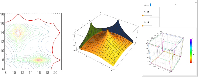
To visualize 4D geometry, I found it most intuitive to use projection. A projection is the distortion of polytopes by scale to lower dimensionality. We can intuitively think about it as the shadow cast by an object. The shadow of a line is a point, the shadow of a polygon is a line, the shadow of a polyhedron is a polygon, and the shadow of a 4-polytope is a polyhedron. As the light source (observer) gets closer from n-dimensional objects, the greater the difference of shadow size between objects. Thus, projection graphs far objects smaller then closer objects.
Here, we plot the shadow of 2D data in 1D (the red line varies in intensity), the projection of 3D data in 2D and the projection of 4D data in 3D (the smaller cube is further away on the fourth dimension):
Out[]=
Geometrical 4D polytopes: Graphics4D
Geometrical 4D polytopes: Graphics4D
Geometrical data visualisation is commonly handled in Mathematica by the Graphics and Graphics3D functions. The goal of such data visualization is to graphs faster and better numerical and geometrical data using powerful human visual pattern recognition capabilities. Yet, with the calculus for 4 dimensional geometry is simple, it has become clear grasping 4D geometry through visualization is very difficult. Rather than focusing on the exact human understanding of 4D spaces, I focused on intuitive ways to view 4D data, relying on human pattern recognition.
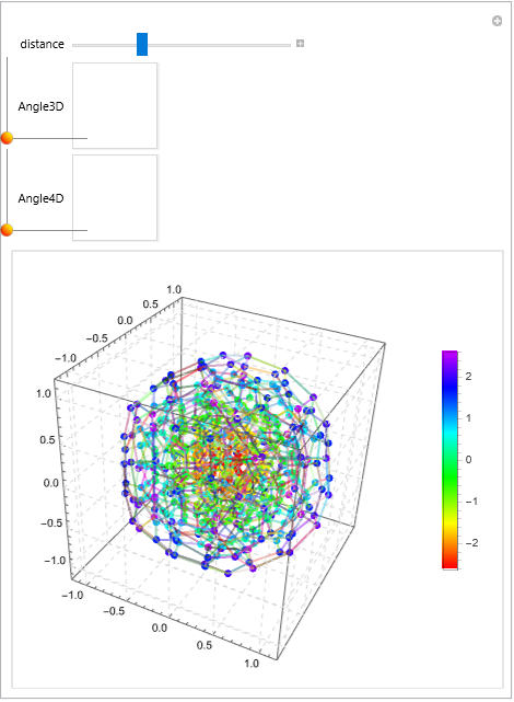
Graphics4D is a representation of four-dimensional data with an interactive 3D graphical image using projection. As it is currently the known best method for 4D visualisation from a 4D observer. Notice the coloring of the points is dependant on the 4th dimension, thus, it should always be considered when observing such data.
Graphics4D is a representation of four-dimensional data with an interactive 3D graphical image using projection. As it is currently the known best method for 4D visualisation from a 4D observer. Notice the coloring of the points is dependant on the 4th dimension, thus, it should always be considered when observing such data.
Familiar interface
Familiar interface
Graphics4D aims to mimic the intuitive interface of Graphics3D and as such has many primitives, namely Point, Line, Triangle, Polygon, Polyhedron, Pentatope, Tesseract, Cell16, Cell24, Cell120 and Cell600, the latter few being regular 4-polytopes, i.e. equivalents semantically to regular polygons and polyhedra.
Plotting the Cell 120 regular 4-polytope:
In[]:=
Graphics4D[{Cell120[{{0,0,0,0},1}]}]
Out[]=
Playful interface
Playful interface
Research tends to indicate the best understanding of 4D space sprouts for deeply interactive visualisation. With this in mind, implementation was geared toward interactivity. Multiple schemes of interaction are available, namely sliders or a gamepad. Thus, with a few list and the data, any 4D geometrical object can be observed, played with and better understood.
A hypercube, triangle and line together. Hands-on challenge: plug-in your gamepad and untangle them! The left joystick controls 3D rotation, while the right joystick controls 4D rotation and left and right of the D-pad controls the distance of the 4D observer. If you don’t have a gamepad, simply change “Gamepad” to “Sliders”:
In[]:=
Graphics4D[Tuples[{-1,1},4]//N,{{1,16},{1,2,6},Range[1,16,2],Range[2,16,2]},{Hue[0],Hue[0.2],Hue[0.1],Hue[0.5]},Controller->"Gamepad"]
Out[]=
Code Initialization
Code Initialization
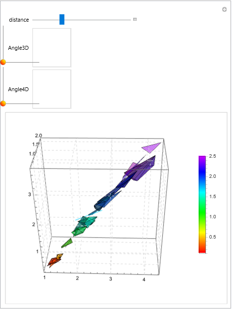
4D data exploration: ListPointPlot4D
4D data exploration: ListPointPlot4D
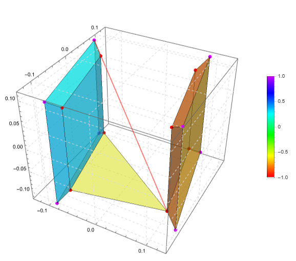
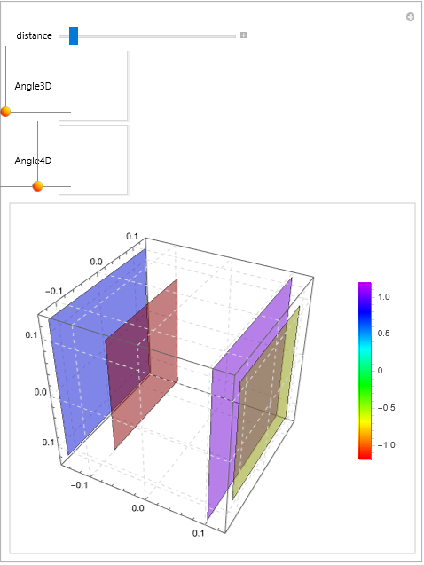
To visualize 4D data in a data science context, it is clear a better adapted function is needed. ListPointPlot4D imitates the ListPointPlot3D function but uses geometry as an advantage. Instead of simply projecting data and coloring it, ListPointPlot4D plots as a single shape all points with the same 4th value. Thus, similar data is grouped and it becomes easy to infer where many points are from the convex shapes created by points.
Seamless polytope construction
Seamless polytope construction
We observe 4D rotation can lead to a continuous change in the distribution of 4th values, making most shapes break into lower dimensionality. This change is expected and the change between polytopes is seamless.
Plotting tesseract points using projection:
In[]:=
ListPointPlot4D[Tuples[{-1,1},4]//N,Method->"Projection"]
Out[]=
Real data exploration
Real data exploration
Thus, through seamless transformation of polytopes and geometric pattern recognition, ListPointPlot4D could become an easy and simple tools to view interaction or tendency in data through all 4 dimensions.
Plotting the iris dataset, specifically the 4 characteristics of each sample as a spacial dimension.
In[]:=
iris=Table[QuantityMagnitude[x],{x,Normal@Values[ResourceData[ResourceObject["Sample Data: Fisher's Irises"]][All,2;;5]]}];ListPointPlot4D[iris]
Out[]=
Code Initialization
Code Initialization
Definition of the ListPointPlot4D
Clear[ListPointPlot4D]Options[ListPointPlot4D]={Method"Projection"};ListPointPlot4D[points_List,OptionsPattern[]]:=Module[{Rotate4D,graphs=Thread[List[Subsets[Range[4],{3}],Reverse[Range[4]]]]},Rotate4D[data_List,xy_,yz_,xz_,xw_,yw_,zw_]:=RotationTransform[2Pixy,{{1,0,0,0},{0,1,0,0}}][RotationTransform[2Piyz,{{0,1,0,0},{0,0,1,0}}][RotationTransform[2Pixz,{{1,0,0,0},{0,0,1,0}}][RotationTransform[2Pixw,{{1,0,0,0},{0,0,0,1}}][RotationTransform[2Piyw,{{0,1,0,0},{0,0,0,1}}][RotationTransform[2Pizw,{{0,0,1,0},{0,0,0,1}}][N[data]]]]]]];If[OptionValue[Method]=="Projection",Manipulate[With[{mat=GroupBy[Rotate4D[points,Angle3D[[1]],Angle3D[[2]],0,Angle4D[[1]],Angle4D[[2]],0],#[[4]]&]},Legended[Graphics3D[Thread[List[Table[Opacity[0.5,x],{x,Hue/@(0.8*Rescale@Keys[mat])}],Table[Thick,Length[mat]],Table[If[MatrixRank[#-First[dimLevel]&/@dimLevel]>=3,ConvexHullMesh[dimLevel],ConvexHullRegion[dimLevel]],{dimLevel,Table[Dot[x[[1]],1/(distance-x[[2]])*IdentityMatrix[{4,3}]],{x,Thread[List[Values[mat],Keys[mat]]]}]}]]],FaceGrids->All,FaceGridsStyleDirective[LightGray,Dashed],Axes->True,TicksAutomatic],BarLegend[{Array[Hue,2,{0,0.8}],{Min[Keys[mat]],Max[Keys[mat]]}}]]],{distance,10,-10},{Angle3D,{0,1},{1,0},ControlType->Slider2D},{Angle4D,{0,1},{1,0},ControlType->Slider2D}],Manipulate[Grid[Partition[Table[With[{mat=GroupBy[Rotate4D[points,Angle3D[[1]],Angle3D[[2]],0,Angle4D[[1]],Angle4D[[2]],0],#[[Last[graph]]]&]},Legended[Labeled[Graphics3D[Thread[List[Table[Opacity[0.5,x],{x,Hue/@(0.8*Rescale@Keys[mat])}],Table[Thick,Length[mat]],Table[If[MatrixRank[#-First[dimLevel]&/@dimLevel]>=3,ConvexHullMesh[dimLevel],ConvexHullRegion[dimLevel]],{dimLevel,Values[mat][[All,All,First[graph]]]}]]],FaceGrids->All,FaceGridsStyleDirective[LightGray,Dashed],TicksAutomatic],StringForm["Dimension `` reduced",Last[graph]],Top],BarLegend[{Array[Hue,2,{0,0.8}],{Min[Keys[mat]],Max[Keys[mat]]}}]]],{graph,graphs}],2]],{Angle3D,{0,1},{1,0},ControlType->Slider2D},{Angle4D,{0,1},{1,0},ControlType->Slider2D}]]]
Conclusions
Conclusions
At first glance, 4D visualization may look difficult and unintuitive. Those 4D visualizations allow better understanding of 4D sparse data using general tools. Both plotting 4D geometry and 4D cloud points for better insights is now possible and more easily interpretable. More efficient implementations of this code are needed for greater dataset exploration. However, the case of dense 4D data remains a difficult task and further tests and prototypes are needed for this task.
Thanks
Thanks
I give my thanks to Connor Gray for accompanying me through all this adventure, Mads Bahrami for believing in me, Silvia Hao for her help with Graphics3D and Stephen Wolfram for guaranteeing the usefulness of this project altogether.