Quantum random walk has striking differences compared to classical random walks. A coin can be a 2D quantum system (like a spin-1/2) and the particle (drunken sailor?) can be treated as a discrete quantum system (eg Hydrogen atom or harmonic oscillator and its energy levels). The coin flip is represented by action of a quantum operator on coin, and up/down (right/left) moves of the particle are determined if the coin is up (eg spin +1/2) or down (eg spin -1/2). In this short computational essay, I will show how to implement quantum random walks in the Wolfram quantum framework.
Intro
Intro
A quantum random walk can be implemented as follows: given a composite system of coin and a particle, flip the coin using a quantum operator, then depending on the coin state, move the particle up/right or down/left. The coin can be a 2D system (eg a spin-1/2) and we shall consider a 2N+1 dimensional Hilbert space for the particle (so with the initial position in the middle and a N-step random walk, the final state will be still in the same Hilbert space). The interesting feature of a quantum random walk is that one does not need to monitor/observe the particle at each step. So at the end, we have a big superposition of all possible trajectories, and each one has a corresponding probability. In fact due to this superposition (and potential interference), the final probabilities are different from classical ones.
This essay is a by-product of a talk I gave at QPitt Quantum Computing Meetup (hosted by my friend, Dr. Daniel Justice). I showed a random walk on a Bloch sphere, and someone asked about this version of quantum random walk (which is, I should say, more interesting, but code wise, a little bit more complicated).
There are interesting references for quantum random walk. I used mostly this one: https://arxiv.org/pdf/quant-ph/0303081.pdf
Install quantum paclet
Install quantum paclet
In[]:=
PacletInstall[CloudObject["https://wolfr.am/DevWQCF"],ForceVersionInstall->True]<<Wolfram`QuantumFramework`
Out[]=
PacletObject
Defining functions for jumping up/down (left/right)
Defining functions for jumping up/down (left/right)
Define an operator that moves up (or right/forward) the particle |i+1〉〈i|
N-1
∑
i=0
In[]:=
jumpUp[n_]:=SparseArray[Table[{If[i+1>n,i-(n-1),i+1],i}->1,{i,n}]]
A peek into one example with n=4
In[]:=
jumpUp[4]//MatrixForm
Out[]//MatrixForm=
0 | 0 | 0 | 1 |
1 | 0 | 0 | 0 |
0 | 1 | 0 | 0 |
0 | 0 | 1 | 0 |
Define an operator that moves down (or left/backward) the particle |i-1〉〈i|
N-1
∑
i=0
In[]:=
jumpDown[n_]:=SparseArray[Table[{If[i==1,n,i-1],i}->1,{i,n}]]
A peek into one example with n=4
In[]:=
jumpDown[4]//MatrixForm
Out[]//MatrixForm=
0 | 1 | 0 | 0 |
0 | 0 | 1 | 0 |
0 | 0 | 0 | 1 |
1 | 0 | 0 | 0 |
Define a function generating random walk, with the inputs as #steps, an operator for coin flipping, and an initial state of the coin
In[]:=
randomWalk[steps_,{coinOp_,coinInitialState_}]:=Module[{n,state,s,u},n=2steps+1;state=QuantumTensorProduct[coinInitialState,QuantumState[SparseArray[{steps+1}->1,{n}],n]];s=QuantumState["0"]["Operator"]@QuantumOperator[jumpUp[n],{2},n]+QuantumState["1"]["Operator"]@QuantumOperator[jumpDown[n],{2},n];u=s@coinOp;NestList[u,state,steps]]
Note that we set the initial position of particle at =#steps and treat it Hilbert space as a -dimensional. So in this way, all possible trajectories will be within possible discrete positions of particle (eg max #steps forward or backwards)
x
0
(2×#steps+1)
To find the corresponding probabilities of finding particle at a position, one can measure the particle’s position and from the result, the corresponding proprieties can be easily extracted
In[]:=
obs[steps_,{coinOp_,coinInitialState_}]:=QuantumMeasurementOperator[QuantumBasis[2steps+1],{2}]/@randomWalk[steps,{coinOp,coinInitialState}]
Exploring some examples
Exploring some examples
In[]:=
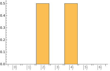
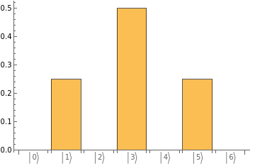
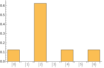
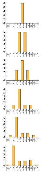
#["ProbabilityPlot"]&/@obs[3,{QuantumOperator["H"],QuantumState["1"]}]//Column
Out[]=
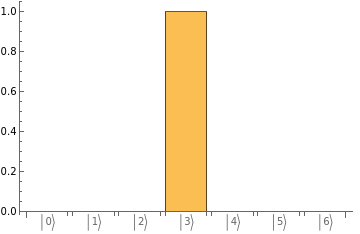
Let’s look at probabilities in a matrix form, which may ilustrates the difference with the classical random walk better (think of binomial distribution and Galton board).
In[]:=
Values[#["Probabilities"]]&/@obs[3,{QuantumOperator[{"XRotation",π/3}],QuantumState["1"]}]//MatrixForm
Out[]//MatrixForm=
0 | 0 | 0 | 1 | 0 | 0 | 0 |
0 | 0 | 3 4 | 0 | 1 4 | 0 | 0 |
0 | 9 16 | 0 | 1 4 | 0 | 3 16 | 0 |
27 64 | 0 | 21 64 | 0 | 7 64 | 0 | 9 64 |
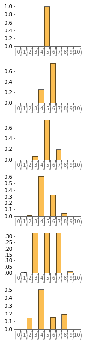
Of course, the way that one flips the coin has a direct effect on the final probabilities. Let’s look at probabilities after 5 steps, where the left column corresponds to Hadamard as the coin-flip, and the right column the X-Rotation as the coin-flip:
In[]:=
GraphicsColumn/@{#["ProbabilityPlot"]&/@obs[5,{QuantumOperator["H"],QuantumState["1"]}],#["ProbabilityPlot"]&/@obs[5,{QuantumOperator[{"XRotation",2π/3}],QuantumState["1"]}]}//Row
Out[]=
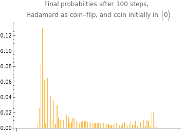
Now let us calculate the probabilities after 100 steps (note the initial state of the coin is and the coin-flip operator is a Hadamard)
|0〉
In[]:=
prop=Diagonal[QuantumPartialTrace[randomWalk[100,{QuantumOperator["H"],QuantumState["1"]}][[-1]],{1}]["DensityMatrix"]];(*Noteprobabilitiescanbecalcualtedlikethistoo:Values[QuantumMeasurementOperator[QuantumBasis[2200+1],{2}][randomWalk[200,{QuantumOperator["H"],QuantumState["1"]}][[-1]]]["Probabilities"]]*)
Plot the corresponding bar chart:
In[]:=
BarChart[prop,PlotLabel"Final probabilties after 100 steps, \n Hadamard as coin-flip, and coin initially in |0〉"]
Out[]=
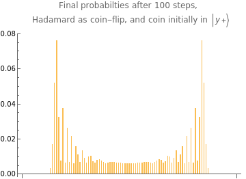
Now let’s add one more interesting quantum feature, with no classical counterpart: the coin is initially in a superposition of 0 and 1 (for example )
|y+〉
In[]:=
prop2=Diagonal[QuantumPartialTrace[randomWalk[100,{QuantumOperator["H"],QuantumState["Right"]}][[-1]],{1}]["DensityMatrix"]];
In[]:=
BarChart[prop2,PlotLabel"Final probabilties after 100 steps, \n Hadamard as coin-flip, and coin initially in |y+〉"]
Out[]=
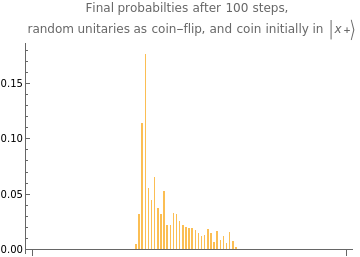
One can explore what happens when the coin is prepared in a different initial state, or with a different coin-flip operator. Additionally, one can randomly change the flip-coin, for example, let pick random unitaries uniformly distributed over U(2) group:
In[]:=
u:=QuantumOperator["RandomUnitary"];prop3=Re@Diagonal[QuantumPartialTrace[randomWalk[100,{u,QuantumState["Right"]}][[-1]],{1}]["DensityMatrix"]];
In[]:=
BarChart[prop3,PlotLabel"Final probabilties after 100 steps, \n random unitaries as coin-flip, and coin initially in |x+〉"]
Out[]=
In other word, calling the quantum particle as a quantum drunken sailor, you have tons of different ways to deal with its drunkenness :D and each treatment will result in a different behaviour (of course) with no classical counterpart, what so ever.