“How many dimensions is our Universe?” Bob asked his friends.
Alice confidently replied, “Don’t be silly, it is 3D!”
Bob, intrigued, countered, “But I watched a video on Sci-A channel stating that according to General Relativity, we live in 3+1D, with the extra dimension being time and holding equal significance to the other three spatial dimensions. Charlie, you’re the expert here, what do you think?”
Charlie, a freshly retired physicist, pondered with a heavy sigh. He then plucked one of Alice’s hairs and remarked, “How many dimensions does this hair have?”...he then continued “ If you’re far enough away, you might think it’s effectively one-dimensional. However, under the microscope, it is 3D. Such might be our Universe.”
Alice, looking confused, asked, “Can you explain more?”
Introduction
Introduction
Exploring the state-of-the-art of phenomena in astrophysics, discernible through advanced observatories like KAGRA, Virgo, LIGO, and the soon-to-be-launched LISA ( also known as NGO), hinges on sophisticated models conducted in 3 +1 dimensions. Most of these models assume our universe to possess three spatial dimensions and one temporal dimension inspired by the framework of general relativity, even if they are constructed within modified theories of gravity, or through semi-classical analysis, attempting to incorporate quantum fields on a curved background, neglecting the backreaction of these fields on the spacetime geometry itself.
Our intuitive perception aligns with a three spatial dimensional universe, it is hard to imagine drawing more than three perpendicular lines at a point. This intuition is supported by stability conditions observed in most solar system orbits and the structure of Maxwell equations [1]. However, theories seeking a quantum version of Einstein’s Gravity, even more trying to unify it with other known interactions, aren’t constrained by this intuition and this number of dimensions. String theory, for example, proposes dimensions far beyond four—up to ten or even twenty-six [2], even if there are some exception to that [4]. Similarly, Kaluza-Klein models necessitate 11 dimensions for grand unifications.
Despite these theories addressing longstanding questions about Quantum Gravity, a crucial consideration is how they operate within the energy scales accessible through experiments or observations (currently a TeV). While many models propose higher dimensions, the observable universe remains 3+ 1 D at our energy scale. String theory, for instance, suggests compactifying the extra dimensions at our energy scale, treating them as effective excitations of a 4D universe . This dynamical dimensionality concept is common in Quantum Gravity theories. On the other hand, some evidence hinting at dimensionality reduction at higher energy scales [4].
Before delving into this dimensionality debate, it’s essential to discuss the utility of scale-dependent dimensions from a classical standpoint. In Sec. I, we’ll explore classical motivations for considering dynamic dimensions. Sec. II will detail how various Quantum Gravity theories, such as Causal Dynamical Triangulation (CDT), and Causal Set Theory incorporate this concept. In Sec. III, our discussion will predominantly draw insights from [2,4], forming the basis for our conclusions. Finally, in Sec. IV, we aim to extend these discussions to contemplate the concept of dimension reduction within the Wolfram Model.”
I. Dimension Reduction from a Classical POV
I. Dimension Reduction from a Classical POV
Recognizing the advantages of altering manifold dimensionality at different scales, an intriguing perspective emerges. This dynamical dimensionality holds implications for both cosmology and particle physics. For a more in-depth exploration of the arguments presented in this section, we strongly encourage the reader to refer to [2].
Higgs
Higgs
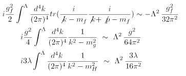
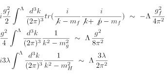
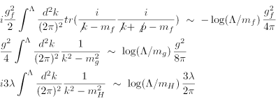
As discussed in [2], lower dimensions exhibit suppressed Ultraviolet divergence in the standard model [5]. For instance, on a Minkowskian background with dimension, n+1, the Higgs field with Yukawa coupling has divergence of for n = 2,3 while Log[Λ] for n=1. The transition from quadratic (linear) divergence to logarithmic divergence as the spatial dimensions shift from three (two) to one is crucial. In that sense, on 1+1 D background, there is no ultraviolet divergence at all, and the theory is super-renormalizable.
Consider the mentioned Lagrangian, we can look the first loop of fermions, gauge bosons and Higgs fields,
n-1
Λ
Consider the mentioned Lagrangian, we can look the first loop of fermions, gauge bosons and Higgs fields,
In[]:=
ToExpression["L_H=D_\\nu \\Phi^{\\dagger} D^\\nu \\Phi-\\mu^2 \\Phi^{\\dagger} \\Phi+\\frac{\\lambda}{2}\\left(\\Phi^{\\dagger} \\Phi\\right)^2-\\sum_f g_f \\Phi \\bar{\\psi}_f \\psi_f",TeXForm]
Out[]=
L
H
∑
f
g
f
ψ
f
ψ
f
2
μ
†
Φ
ν
D
D
ν
†
Φ
1
2
2
Φ
2
()
†
Φ
where Φ is the Higgs field, = λ= , and are the fermion and Higgs mass respectively, while ν is the Higgs field vacuum expectation value. is the covariant derivative for the field.
2
g
f
2
m
f
2
ν
2
m
H
2
2
ν
m
f
m
H
ν
D
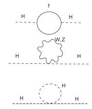
Applying the Feynman rules to those digrams one find the cut off momentum ( conversely energy) scale Λ, one obtain the following integrals in three, two and one spatial dimensions respectively.
QCD
QCD
Quantum Chromo Dynamics (QCD) is also super-renormalizable in 2+1 D and 1+1 D, obviating the need for lattice regularization common in 3+1 D. The shift in dimensionality will make QCD coupling constant has a positive dimension, facilitates convergence in perturbative schemes akin to Quantum Electro Dynamics (QED).
ToExpression[" \\mathcal{L}=-\\frac{1}{4} F_{\\mu \\nu}^a F^{a \\mu \\nu}+i \\bar{\\psi} \\gamma^\\mu\\left(\\partial_\\mu+i g A_\\mu^a T^a\\right) \\psi \\\\ ",TeXForm]ToExpression[" F_{\\mu \\nu}^a=\\partial_\\mu A_\\nu^a-\\partial_\\nu A_\\mu^a+g f^{a b c} A_\\mu^b A_\\nu^b",TeXForm]
L-+i(ψ)
1
4
aμν
F
a
F
μν
D
μ
ψ
μ
γ
a
F
μν
∂
μ
a
A
ν
∂
ν
a
A
μ
abc
f
b
A
μ
c
A
ν
Moreover in the same way dimension reduction can cure Ultraviolet divergence at higher energy scales, dimension construction could be used to cure infrared divergence. The reader can find an example illustrated in [2] Sec I. 5.
Cosmology
Cosmology
Illustratively, we can also consider the utility of dimension reduction in a cosmological model. By solving Einstein Field equations in 4+1 D and regarding our universe as a hypersurface in 3+1 D, one can account for the cosmological constant from a geometric point of view. For someone living in our universe, a hypersurface on the 4+1 D, a effective stress-energy tensor will be detectable, this could be used to the recovery of the well-known FRLW metric.
In[]:=
<<OGRe`
OGRe:
OGRe: An Object-Oriented General Relativity Package for Mathematica |
v1.7.0 (2021-09-17) |
• To view the full documentation for the package, type |
• To list all available modules, type |
• To get help on a particular module, type ? followed by the module name. |
• To enable parallelization, type |
• OGRe`Private`UpdateMessage To disable automatic checks for updates at startup, type |
TNewCoordinates["Spherical5D",{t,r,θ,ϕ,ψ}]TNewCoordinates["Spherical4D",{t,r,θ,ϕ}]
Clear[Λ,ψ]
TNewMetric"Universe5D","Spherical5D",{1,0,0,0,0},0,-Exp2t,0,0,0,0,0,-Exp2t,0,0,0,0,0,-Exp2t,0,{0,0,0,0,-1}TNewMetric"FLRW","Spherical4D",{1,0,0,0},0,-Exp2t,0,0,0,0,-Exp2t,0,0,0,0,-Exp2tTNewMetric["FLRWTraditional","Spherical4D",{{1,0,0,0},{0,-,0,0},{0,0,-,0},{0,0,0,-}}]
Λ[ψ]
3
2
r
Λ[ψ]
3
2
r
2
Sin[θ]
Λ[ψ]
3
Λ[ψ]
3
2
r
Λ[ψ]
3
2
r
2
Sin[θ]
Λ[ψ]
3
2
a[t]
2
r
2
a[t]
2
r
2
Sin[θ]
2
a[t]
In that sense we can recognize the flat (k=0) FLRW as a hypersurface of the 4+1 D universe through examining the slice of = . We wrote also the FLRW metric in the convenient way to make it easy to recognize the scale factor a(t)
2
ψ
3
Λ
In[]:=
TShow["Universe5D"]TShow["FLRW"]TShow["FLRWTraditional"]
OGRe:
Universe5D: (t,r,θ,ϕ,ψ) =
g
μν
1 | 0 | 0 | 0 | 0 |
0 | - 2t Λ[ψ] 3 | 0 | 0 | 0 |
0 | 0 | - 2t Λ[ψ] 3 2 r | 0 | 0 |
0 | 0 | 0 | - 2t Λ[ψ] 3 2 r 2 Sin[θ] | 0 |
0 | 0 | 0 | 0 | -1 |
OGRe:
FLRW: (t,r,θ,ϕ) =
g
μν
1 | 0 | 0 | 0 |
0 | - 2t ψ | 0 | 0 |
0 | 0 | - 2t ψ 2 r | 0 |
0 | 0 | 0 | - 2t ψ 2 r 2 Sin[θ] |
OGRe:
FLRWTraditional: (t,r,θ,ϕ) =
g
μν
1 | 0 | 0 | 0 |
0 | - 2 a[t] | 0 | 0 |
0 | 0 | - 2 r 2 a[t] | 0 |
0 | 0 | 0 | - 2 r 2 a[t] 2 Sin[θ] |
Also we can write down the effective induced matter tensor =κ, where κ is a constant.
μν
T
μν
G
TList[TCalcEinsteinTensor["FLRW"]]
OGRe:
FLRWEinstein: | ||||||||||||
|
II. Dimension Reduction, a trend in Quantum Gravity Theories
II. Dimension Reduction, a trend in Quantum Gravity Theories
As highlighted in the introduction, there exists a discernible trend in various models of Quantum Gravity, wherein the dimensionality undergoes reduction at elevated energy scales or, conversely, when probing distances on the order of the Planck length . This section will delve deeper into this phenomenon, drawing extensively from [4] and [2] to shed light on these intriguing aspects within the existing literature. In this report, our focus will be exclusively on Causal Dynamical Triangulations and Causal Set theory. Additionally, we will touch upon asymptotic safety theories as part of the conclusion. However, readers interested in exploring this trend further can find additional insights in loop Quantum Gravity, non-commutative gravity theories, and more in [2,4].”
l
p
Causal Dynamical Triangulations (CDT)
Causal Dynamical Triangulations (CDT)
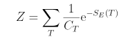
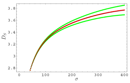
CDT is a path integral formalism of quantum gravity that employs a discrete approach to model the dynamical evolution of spacetime. Although CDT doesn’t make any assumptions about the nature of the spacetime itself, still it utilize an artificial lattice configuration on the geometry of interest, dividing the spacetime into simplicial building blocks, a generalized version of triangles in 2D, and the configuration of these building blocks evolves dynamically. Crucially, the evolution adheres to causal constraints in other words some of those edges are timelike in contrast with the Euclidean Dynamical triangulation (EDT) at which all edges are spacelike. This ensure the exclusion of the non-lorentzian possible configurations. Analytically handling CDT for dimensions higher than 1+1 D poses challenges, prompting a reliance on numerical tools such as Monte Carlo simulations. These simulations facilitate the computation of the path integral, summing over the myriad possible geometric configurations. This approach provides a powerful tool for exploring the quantum characteristics of spacetime within the CDT framework [5].where is a combinatorial symmetry factor and (T) is the Einstein- Regge action of the triangulation after the wick rotation is preformed. One of the physical and mathematical measures of dimensions in CDT is the spectral dimension . In [7], Ambjørn, Jurkiewicz, and Loll stumbled upon a surprising revelation. While the anticipated value for the was 4 at larger scales, essentially almost mimicking a four-dimensional universe over considerable distances, the model exhibited an unforeseen decline to around ≈ 2 at smaller scales. The same phenomena happen when 2+1 D CDT applied the approaches 3 at large scale while drop to ≈ 2 at smaller scales. This scenario is traced back to phase transition in the dominating geometries withing the path sums; it is believed that at low scales the configurations of more fractal nature overwhelm others, still at higher scales more continuous structure take over allowing for manifold like structure [4].It’s noteworthy that while the author employs the terminology of a phase transition, the cascade of dimensional changes is gradual, lacking abrupt jumps typically associated with the conventional notion of a phase transition.
C
T
S
E
d
s
d
s
d
s
d
s
d
s
D
s
D
s
4.02−
119
54+σ
Once more, this aligns seamlessly with the overarching theme of this report— the reduction of dimensions at higher energy scales implies the potential for more renormalizable theories; wether we are considering quantum gravity theory or QFTs coupled with it. As articulated in [7], “It is natural to conjecture it will provide an effective short-distance cut-off by which the non-perturbative formulation of quantum gravity employed here, causal dynamical triangulations, evades the ultraviolet infinities of perturbative quantum gravity.”
Causal Set Theory
Causal Set Theory
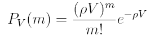
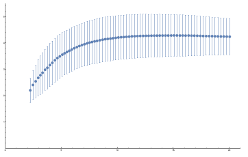
The essence of the causal set theory approach to quantum gravity lies in the pursuit of discretizing spacetime. While the intricate structure of a manifold is far more sophisticated than a mere collection of sets, causal set theory endeavors to illuminate quantum aspects of gravity by discarding the wealth of information encoded in the manifold structure, retaining only the crucial causal relationships among its points. Most causal sets do not exhibit manifold-like structure, therefore a more viable approach top-down one. The task of finding a causal set that approximates a given manifold is relatively straightforward. This is achieved through a process called “sprinkling,” involving the random distribution of points via a Poisson process. This obviously persevere the lorentzian signature of the geometry in terms of partially ordered sets of points. Notably, the density of the sprinkling plays a pivotal role in shaping the resemblance to a continuous structure. As the sprinkling becomes more dense, the resulting causal set progressively mirrors the manifold-like characteristics- including curvature measures. Where the probability of finding m points in any volumes V at a discrete scale given byThis eqSprinkling of 3+1 D Minkowski space in [8], the dimension of the sets was measured as a function of the density of points. The Myrheim-Meyer dimensions was employed for those purposes; which is basically counting the causal relations between the points. The reader can find more details on this measure in [8] and [4]. Dense sprinkling approached dimension of 4 for the case of Minkowski manifold. The dimensions we studied, we found that dimensional reduction does indeed occur as the volume decreases. The descent into lower dimensions initiates at a volume proportional to the dimensionality of the n+1-dimensional Minkowski manifolds. Below this transition point, the reduction becomes notably swift, the consistently diminishes to 2. The reader can find an exception to that at which the dimension reduces to zero as reported in [8].Myrheim-Meyer dimension in a four-dimensional background at different scale [8].
-1
ρ
d
MM
d
MM
III. Conclusion and Discussion
III. Conclusion and Discussion
At this juncture, the reader might be grappling with numerous questions surrounding the pervasive trend of dimension reduction in aspiring quantum gravity theories. What imparts uniqueness to gravity in 1+1 dimensions? Is the phenomenon could formulated in terms of renormalization? While concrete answers remain elusive in the absence of a comprehensive quantum gravity theory, intriguing speculations that align coherently with theoretical arguments have been proposed [4, 2].
Scale Invariance
Scale Invariance
Let’s delve into the realm of 1+1 dimensional gravity. In this context, the Einstein-Hilbert Action is solely contingent on the topological (global) features of the manifold, the action in that is only the Euler characteristic of the manifold [2]. This implies a lack of local- wether curvature or fluctuations namely Gravitational waves or Gravitons- measures in the theory. Conversely, the gravitational coupling constant G is dimensionless and consequently endowing the theory with scale invariance—insensitivity to energy scales.
In terms of renormalization, 1+1 dimensional gravity exhibits a non-Gaussian UV fixed point, suggesting that reliability as a quantum gravity theory may hinge on the deliberate loss of sensitivity to energy scale, with dimension reduction as a mechanism for that. In the language of quantum field theory, this aligns with the asymptotic safety theory of gravity, although there is currently no empirical evidence supporting General Relativity as such a theory. Moreover, this intriguing scale invariance feature can also be explored within the realm of CDT, where phase transitions reveal scales at which dimension reduction becomes notably pronounced. Post-transition, the theory approaches its continuum limit, with a predisposition towards scale invariance—a coherence that resonates with the renormalization argument presented [4].
In terms of renormalization, 1+1 dimensional gravity exhibits a non-Gaussian UV fixed point, suggesting that reliability as a quantum gravity theory may hinge on the deliberate loss of sensitivity to energy scale, with dimension reduction as a mechanism for that. In the language of quantum field theory, this aligns with the asymptotic safety theory of gravity, although there is currently no empirical evidence supporting General Relativity as such a theory. Moreover, this intriguing scale invariance feature can also be explored within the realm of CDT, where phase transitions reveal scales at which dimension reduction becomes notably pronounced. Post-transition, the theory approaches its continuum limit, with a predisposition towards scale invariance—a coherence that resonates with the renormalization argument presented [4].
Asymptotic Silence
Asymptotic Silence
According to [2,4], an alternative explanation for this trend involves the concept of Asymptotic Silence. To provide context, envision a generic space singularity influenced by strong gravity, concentrating light in all directions—in modern gravity language as the light cone will close up. This leads to the shrinking of particle horizons, impeding communication between timelines. In cosmology, this scenario is termed Asymptotic Silence.At the Planck length , Asymptotic Silence is expected among local spacetime regions. With being finite, it’s reasonable to infer universe of more then one dimension at that scale. In [4], the author traced this back to the decoupling of neighboring points ; leads to BKL behavior in 1+1 D. Asymptotic silence was reported in both the framework of set theory and loop quantum gravity.
l
p
l
p
IV. On the Wolfram Model
IV. On the Wolfram Model
The Wolfram Physics Project endeavors to uncover a fundamental theory of physics by proposing a novel approach rooted in simple rules within a hypergraph framework. In this conceptualization, the vertices of these hypergraphs represent space atoms that undergo evolution governed by specified rewriting rules. This approach disrupts the equivalence between spatial and temporal dimensions, drawing parallels with causal set theory mentality. The measure of dimension ,named the wolfram Hausdorff Dimensions, of the spacetime in that case is the connectivity of the graph itself which is again similar to the measure. If we agreed to some extend that , , and are all reliable and conceptually relatable measures of dimensions in WM, CST and CDT respectively.
d
WH
d
MM
d
WH
d
MM
d
s
Sketch for Asymptotic Silence in WM
Sketch for Asymptotic Silence in WM
This will motivate searching for such dimension reduction scenarios within WM, to be more accurate; evolving dimension ones as those hyper graphs usually starts with low-scale spatial universe. For example, if we tried to apply this concept of asymptotic silence to hypergraphs, would involve searching for network of locally connected subgraphs; still they are disconnected at larger domains. On average if of subgraphs is around 2. Still, as the scale build up a phase transition in the connectivity will be necessary to evolving the dimension of the hypergraph globally.
Unfortunately, the author is currently unaware of any updating rules that closely resemble such a universe. Nevertheless, this aspect can be addressed in future work.
d
WH
Unfortunately, the author is currently unaware of any updating rules that closely resemble such a universe. Nevertheless, this aspect can be addressed in future work.
Can we have Bottom-Top approach for WM?
Can we have Bottom-Top approach for WM?
Perhaps a more robust method for studying dimension reduction in WM would involve approximating solutions to the Einstein Field equation at various scales and quantifying the connectivity of the causal hypergraph among its vertices. While resembling the approach of CST, this method will reply measures not of the hypergraph itself but of its causal dual. Still the questions of how to achieve so is highly non-trivial, one potential starting point could be to explore the desiccation procedure outlined in [9].
d
WM
Acknowledgments
Acknowledgments
I extend my sincere gratitude to my mentors, Xerxes D. Arsiwalla and Hatem Elshatlawy, for their invaluable guidance and support during the winter school. Their expertise and mentorship have greatly enriched my learning experience. Additionally, I would like to express my thanks to all the organizers, speakers, and Stephen Wolfram for their dedicated effort and time.
References
References
[1] P. Ehrenfest, KNAW Proc. 20 I (1918) 200.
[2] Stojkovic, D. (2014). “Vanishing dimensions: Review.” arXiv preprint arXiv:1406.2696.
[3] Graña, M., & Triendl, H. (2017). String theory compactifications. SpringerBriefs in Physics, 1–74. https://doi.org/10.1007/978-3-319-54316-1_1
[4] Carlip, S. (2017). “Dimension and dimensional reduction in quantum gravity.” Classical and Quantum Gravity, 34(19), 193001. doi:10.1088/1361-6382/aa8535
[5] Peskin, M. E., & Schroeder, D. V. (1995). An introduction to quantum field theory. Perseus Books.
[6] Loll, R. (2019). “Quantum gravity from causal dynamical triangulations: a review.” Classical and Quantum Gravity, 37(1), 013002. doi:10.1088/1361-6382/ab57c7
[7] Ambjørn, J., Jurkiewicz, J., & Loll, R. (2005). “The Spectral Dimension of the Universe is Scale Dependent.” Physical Review Letters, 95(17), 171301. doi:10.1103/PhysRevLett.95.171301
[8] Abajian, J., & Carlip, S. (2018). “Dimensional reduction in manifoldlike causal sets.” Physical Review D, 97(6), 066007. doi:10.1103/PhysRevD.97.066007
[9] Khatsymovsky, V. M. (2020). “On the discrete version of the black hole solution.” International Journal of Modern Physics A, 35(11n12), 2050058. doi:10.1142/S0217751X2050058X
CITE THIS NOTEBOOK
CITE THIS NOTEBOOK
How many dimensions are there? Dynamical Dimensions & Dimension Reduction
by Fawzi Aly
Wolfram Community, STAFF PICKS, January 11, 2024
https://community.wolfram.com/groups/-/m/t/3101823
by Fawzi Aly
Wolfram Community, STAFF PICKS, January 11, 2024
https://community.wolfram.com/groups/-/m/t/3101823