Causal set theory is a combinatorial theory of quantum gravity that describes spacetime as a partially ordered set. Since causal set theory is based on finite structures, arguments and evidence is required to recover properties described by quantum mechanics and general and special relativity. A large part of the summer program was teaching myself causal set theory and I strived to keep this presentation self-contained and used Mathematica to give an interactive introduction. I hope that those new to the subject will benefit the most. For those who know causal set theory, we offer more efficient Mathematica routines than were previously available for working with causal sets and show how to use this code to investigate the convergence rate of the Gromov-Hausdorff distance between open sets of causal sets and open sets in Minkowski spacetime. We end with brief remarks on how topology relates to Wolfram Model rules.
Topological Spaces
Topological Spaces
Topological spaces are minimal models of space that play a foundational role in modern mathematics. For our purposes, this introduction to topology will help us understand causal set theory. The route we take follows the path laid out in 1937 by Soviet mathematician Pavel Alexandroff. It’s an important path because topology facilitates the introduction of spatial structures in situations that are not obviously spatial at the outset. We take the rather traditional approach by defining a topological space as a special collection of subsets of an underlying set. This collection of subsets is then used to characterize everyday concepts like convergence, continuity, and nearness. From a physical perspective, we can imagine topology as the subject which analyzes the relation between points and boundaries. We’ll see shortly that boundaries demarcating what is near what are called open sets. A good collection of these open sets will define a data structure describing in what sense a point is close by another point. A topology brings cohesion and minimal harmony to an otherwise barren collection of things. A unique aspect of this presentation is the use of Mathematica to introduce and manipulate topological structures. So please play with the code to get a feel for things.
It’s Never Too Late to Topologize
It’s Never Too Late to Topologize
Definition 1.1. A topology on X consists of a set τ of subsets of X, called the “open sets of X in the topology τ ”, satisfying the following requirements.
(i) ∅ and X are in τ .
(ii) A finite intersection of sets in τ is in τ .
(iii) An arbitrary union of sets in τ is in τ .
The pair (X, τ) is called a topological space. The first axiom exists so that intersections and unions are adequately closed. There is a generalization that will become important later in one’s study. We introduce it now by loosening up the finiteness restriction on the second axiom.
Definition 1.2. An Alexandroff space is a topological space for which arbitrary intersections of open subsets are still open.
We immediately notice that every finite topological space is an Alexandroff space. One later learns that Alexandroff spaces are equivalent to infinite posets but we leave it at that for now. Let’s keep our attention on good-old fashion finite topological spaces. We define these structures in Mathematica by specify open sets and checking the required properties.
In[]:=
On[Assert];SetAttributes[set,Orderless];set[elms___]:=With[{nodups=DeleteDuplicates@{elms}},set@@nodups/;{elms}=!=nodups]FiniteTopologicalSpace[elements_List,topology_List]:=Module[{makeSet},makeSet=List@@set[Union[Sort/@topology]];<|"Points"elements,"OpenSets"First[makeSet]|>];FiniteTopologicalSpaceQ[topologicalSpace_Association]:=Module[{elements,topology,collectionOfSets,axiomOne,axiomTwo,axiomThree},elements=topologicalSpace["Points"];topology=topologicalSpace["OpenSets"];axiomOne=MemberQ[topology,elements]&&MemberQ[topology,{}];collectionOfSets=Select[Subsets[topology],(#!={})&];axiomTwo=AllTrue[Union[Intersection@@@collectionOfSets],MemberQ[topology,#]&];axiomThree=AllTrue[Union[Union@@@collectionOfSets],MemberQ[topology,#]&];{axiomOne,axiomTwo,axiomThree}];
Create a topological space and check the axioms
X={1,2,3};τ={{},{1},{2},{3},{1,2},{1,3},{3,2},{1,2,3}};topologicalSpace=FiniteTopologicalSpace[X,τ]FiniteTopologicalSpaceQ[topologicalSpace]=={True,True,True};
Out[]=
Points{1,2,3},OpenSets{{},{1},{2},{3},{1,2},{1,3},{2,3},{1,2,3}}
Generating Topologies Without Thinking
Generating Topologies Without Thinking
Once X becomes sufficiently large, it’s cumbersome to specify every open set explicitly. So we need a easier way of creating topological space. This desire gives rise to the following definition.
Definition 1.3 Let (X,τ) be a topological space. A subbase, aka subbasis, of τ is defined as a subcollection S of τ such that any other topology τ’ on X containing S must also contain τ. When this happens, we say that τ is the smallest topology containing S.
There is a more computationally practical characterization of a subbasis, and like all fact of mathematics, it’s a theorem. In this presentation, we offer some proofs and neglect others. This decision was made because of time considerations, and one could imagine a proper presentation in the future. Nonetheless, we point readers to references whenever I can remember.
Proposition 1.1. Let X be a set and let S be any collection of subsets of X such that that union of all subsets of S equal X.
If T is the set of all subsets of X created in the following ways:
1) finite intersections of sets in S;
2) all unions of sets obtained in 1),
Then T is a topology on X.
With this proposition in mind, we can think of a subbasis as a collection of sets that can be fixed up into a valid topological space in a minimal way. The topology defined in the previous proposition is called the topology generated by S, and the collection S is called a subbasis for the topology. So for any subcollection S of the power set, there is a unique topology that has S as a subbasis. This idea will come up again at the end when we look at Wolfram model rules. But for now, it’s important to realize that, in general, there is no unique subbasis for a topology. If we start with a topology, there could be a ton of ways to produce it, but if we start with a collection of subsets, we can enlarge it in a unique way to get a topology.
Generate a topological space from a subbasis
In[]:=
GenerateTopologyFromSubBasis[subBasis_List]:=Module[{collectionOfSets,elements,finiteIntersections,unions,topology},elements=Union@@subBasis;collectionOfSets=Select[Subsets[subBasis],(#!={})&];finiteIntersections=Union[Intersection@@@collectionOfSets];unions=Union@@@Subsets[finiteIntersections];topology=Union[finiteIntersections,unions];FiniteTopologicalSpace[elements,topology]];
S={{a,b,c},{b,c,d}};τ=GenerateTopologyFromSubBasis[S]FiniteTopologicalSpaceQ[τ]=={True,True,True}
Out[]=
Points{a,b,c,d},OpenSets{{},{b,c},{a,b,c},{b,c,d},{a,b,c,d}}
Out[]=
True
Base for a Space
Base for a Space
The above construction allows us to create a new topology from any collection of sets. The flexibility of a subbasis comes at the cost of knowing what the final open sets are in the generated topology. It’s difficult to discern all the open sets when given just a subbase without explicitly generating the entire topological space and checking. Fortunately, there is a middle ground between specifying every open set and working with an arbitrary collection of subsets of the powerset. Another compressed description of a topological space only writes down the alphabet of open sets. In this style of description, a topological structure is given by the parts that are sufficient to generate the topological structure.
Definition 1.4 . Base or basis for a topological space (X, τ) is a family B of open subsets of X such that every nonempty open set of the topology is equal to a union of sets belonging to B .
Like before, we have a more intrinsic definition that is operationally useful. Notice that the following two conditions are required to ensure that the set of all unions of subsets of B is a topology on X:
The base elements cover X:b = X
Let, be base elements and x in ∩, then there is a base element such x ∈ ⊂ ∩
So, an alternative definition of a base is a collection B of open subsets of X satisfying the above properties. A base is not always a topology, but we can grow a basis into a topology.
Proposition 1.2. Let B is a base. There is a recipe for creating the topology determined by a base:
τ = {unions of elements of B} = { : ∈ B }
And τ is the smallest topology containing B.
Definition 1.4 . Base or basis for a topological space (X, τ) is a family B of open subsets of X such that every nonempty open set of the topology is equal to a union of sets belonging to B .
Like before, we have a more intrinsic definition that is operationally useful. Notice that the following two conditions are required to ensure that the set of all unions of subsets of B is a topology on X:
The base elements cover X:
U
b∈B
Let
B
1
B
2
B
1
B
2
B
3
B
3
B
1
B
2
So, an alternative definition of a base is a collection B of open subsets of X satisfying the above properties. A base is not always a topology, but we can grow a basis into a topology.
Proposition 1.2. Let B is a base. There is a recipe for creating the topology determined by a base:
τ = {unions of elements of B} = {
U
i
b
i
b
i
And τ is the smallest topology containing B.
Check if the provided collection of sets is a base and then generate a topological space from a base
In[]:=
BaseQ[base_List]:=AllTrue[Table[AnyTrue[#,TrueQ]&@@Table[Table[SubsetQ[intersectedSet,basicSet]&&MemberQ[basicSet,x],{basicSet,base}],{x,intersectedSet}],{intersectedSet,Select[Union[Intersection@@@Subsets[base,{2}]],(#!={})&]}],TrueQ];GenerateTopologyFromBase[base_List]:=Module[{covering,topology},covering=Union@@base;topology=Insert[Union@@@Subsets[base],{},-1];FiniteTopologicalSpace[covering,topology]];
Here are examples which are not a bases.
base={{a,b,c},{b,c,d}};BaseQ[base]GenerateTopologyFromBase[base]τ=FiniteTopologicalSpaceQ[GenerateTopologyFromBase[base]]base={{0,1},{0,2}};BaseQ[base]GenerateTopologyFromBase[base]τ=FiniteTopologicalSpaceQ[GenerateTopologyFromBase[base]]
Out[]=
False
Out[]=
Points{a,b,c,d},OpenSets{{},{a,b,c},{b,c,d},{a,b,c,d}}
Out[]=
{True,False,True}
Out[]=
False
Out[]=
Points{0,1,2},OpenSets{{},{0,1},{0,2},{0,1,2}}
Out[]=
{True,False,True}
Here’s an example of a collection of sets that is a base.
base={{0},{0,1},{0,2}};BaseQ[base]GenerateTopologyFromBase[base]τ=FiniteTopologicalSpaceQ[GenerateTopologyFromBase[base]]
Out[]=
True
Out[]=
Points{0,1,2},OpenSets{{},{0},{0,1},{0,2},{0,1,2}}
Out[]=
{True,True,True}
Between A Rock and A Hard Place
Between A Rock and A Hard Place
In causal set theory, special attention is placed on a base for a particular type of topology called the interval topology or Alexandroff topology. Unfortunately, these names are used interchangeably in causal set theory. In this work, we differentiate between them. We will use the interval topology to denote the topology commonly used in causal set theory. This interchanging of names is understandable because both structures naturally arise when dealing with orders.
The first ordering on a set we learn about is the preorder, and the natural topology that arises from the preorder is called the Alexandroff topology. The second kind of order is a partial order, and this gives way to the interval topology.
Definition 1.5. A preorder on a set S is a reflexive and transitive relation, denote by ≺. We call (S, ≺) preordered set.
Definition 2.1. Let P be a preordered set.
Declare a subset A of P to be an open subset if x≺y and x∈A, then y∈A. This defines a topology on P, called the specialization topology or Alexandroff topology. We write this topology symbolically as τ ={A⊆ X : ∀ x,y∈ X (x∈ A ∧ x ≺ y) → y∈ A}
Now now we define the interval topology that is commonly used in causal set theory. A preorder is a partial order if it is antisymmetric, i.e., x ≤ y and y ≤ x imply that x = y. A set X with a partial order (X,≤) is called a poset.
Let (X, ≤) be a poset with at least two elements. Then interval topology on X is the smallest topology in which subsets of X, called intervals, having the
forms
[a] = {x ∈ X | a < x}, for all a in X, called right rays, chronological future, or future light cones
•[a] = {x ∈ X | x < a}, for all a in X, called left rays, chronological past, or past light cones
• <<a,b>> =[a] ∩ [b] = {x ∈ X | a < x < b}, for all a and b in X,
are open sets.
This is a base for a topological structure. The topology determined by this base is the interval topology, aka order topology, of the partially ordered set (X, ≤). We can work with examples interactively in Mathematica. Moreover, to do so, it’s often convenient to consider a partially ordered set as a graph whose vertex set is X with edges connecting two vertices if they satisfy the partial order. We use terms like “chronological future,” “chronological past,” and “future light cones” above to introduce the flavor of causal set theory.
The first ordering on a set we learn about is the preorder, and the natural topology that arises from the preorder is called the Alexandroff topology. The second kind of order is a partial order, and this gives way to the interval topology.
Definition 1.5. A preorder on a set S is a reflexive and transitive relation, denote by ≺. We call (S, ≺) preordered set.
Definition 2.1. Let P be a preordered set.
Declare a subset A of P to be an open subset if x≺y and x∈A, then y∈A. This defines a topology on P, called the specialization topology or Alexandroff topology. We write this topology symbolically as τ ={A⊆ X : ∀ x,y∈ X (x∈ A ∧ x ≺ y) → y∈ A}
Now now we define the interval topology that is commonly used in causal set theory. A preorder is a partial order if it is antisymmetric, i.e., x ≤ y and y ≤ x imply that x = y. A set X with a partial order (X,≤) is called a poset.
Let (X, ≤) be a poset with at least two elements. Then interval topology on X is the smallest topology in which subsets of X, called intervals, having the
forms
+
•I
•
-
I
• <<a,b>> =
+
I
-
I
are open sets.
This is a base for a topological structure. The topology determined by this base is the interval topology, aka order topology, of the partially ordered set (X, ≤). We can work with examples interactively in Mathematica. Moreover, to do so, it’s often convenient to consider a partially ordered set as a graph whose vertex set is X with edges connecting two vertices if they satisfy the partial order. We use terms like “chronological future,” “chronological past,” and “future light cones” above to introduce the flavor of causal set theory.
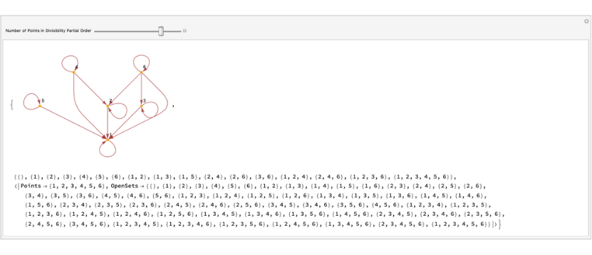
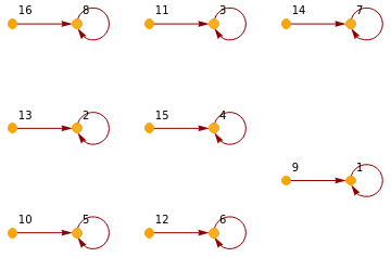
Create the base for the interval topology using the partial order given by divisibility and then generate the interval topology using the base.
In[]:=
+
I
-
I
+
I
-
I
In[]:=
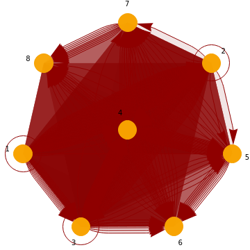
anim=Manipulate[divisibilityGraph=RelationGraph[(Mod[#1,#2]==0)&,Range[i],VertexLabels->"Name",VertexStyleDirective[Hue[0.11,1,0.97],EdgeForm[{Hue[0.11,1,0.97],Opacity[1]}]],EdgeStyleHue[0,1,0.56]];X=VertexList[divisibilityGraph];rightRays=Table[[divisibilityGraph,a],{a,X}];leftRays=Table[[divisibilityGraph,a],{a,X}];closedInterval=Union[IntervalBasicOpenSet[divisibilityGraph,#[[1]],#[[2]]]&/@Tuples[X,2]];base=DeleteDuplicates[Sort/@Union[rightRays,leftRays,closedInterval]];Assert[BaseQ[base]];{divisibilityGraph,base,GenerateTopologyFromBase[base]},{{i,2,"Number of Points in Divisibility Partial Order"},2,7,1}]
+
I
-
I
frames=Import[Export["divisibilityGraph.gif",anim]];ListAnimate[ImageResize[#,1000]&/@frames]
Out[]=
When is one thing equal to some other thing?
When is one thing equal to some other thing?
Before going on to causal set theory, let’s think about the physical consequences of our current definition of a topological space and how to faithfully illustrate these spaces. Thus far, our description of topology has been visually improvised. However, we can change this by thinking about the following question: To what extent can points can be distinguished from each other by only considering the regions which hold then? From the viewpoint of physics, this line of thought is related to the idea that if (X, τ) is a model of physical space, then any real object must exist inside some region of space. But what should we do if two points belong to the same collections of open sets? Should we consider these to be the same? How do we determine which topologies make this distinction and which ones do not?Here’s one relevant mathematical concept to helps us see which topologies distinguishes points: For any two points x,y in X, there is an open set U such that x in U and y not in U or y in U and x not in U. We call the above condition the T0 separation axiom. Some spaces satisfy it, and some don’t. Topological spaces that do are called T0-spaces, Alexandroff T0-space, or Kolmogorov spaces. There are other separations axioms, but we’ll concern ourselves only with this one for now. For those in the know, I should point out that any finite topological space can transformed into a T0 space so they are same from the perspective of homotopy. Recalling some earlier definitions, let’s create a partially ordered from a T0-space and then do the magic trick and go the other direction. This story probably goes back to Pavel Alexandroff, but I heard from it from Peter May. I think he heard it from Micheal McCord's and Robert Strong's work during the 60s. For experienced riders, we are scratching the surface and won’t get to the fun parts of homotopy. For those who are new, welcome! This is where it all starts. Let be the intersection of all open sets containing x in (X, τ). Proposition 1.3. The collection of open sets {:xinX} is the unique minimal base for X. Starting with a topological space satisfying the T0 separation axiom, we can turn this into a partially ordered set. Define the following relation ≤ on an T0-space X: x ≤ y whenever ⊂ . Notice that ≤ is reflexive and transitive, so at the very least, we know that (X ,≤ ) is a preordered set. We haven’t used the fact that we started with a T0-space. That comes into play when we notice that if x≤y and y≤x, then = because the space distinguishes points, every open set containing either x or y must also contain the other point. So the T0 separation axiom implies that ≤ is antisymmetric. Therefore, (X ,≤ ) is a poset. This correspondence allows us to visualize T0 topological spaces with the following Mathematica code. Given a partial order, its Hasse diagram is a directed graph whose vertex set is X and edges are (x, y) satisfying the order but where there exist no elements in between.
U
x
U
x
U
x
U
y
U
x
U
y
Transform a topological space into a partially ordered set using the method outlined above.
In[]:=
topologyRelationCondition[intersectionSets_Association]:=Function[{x,y},SubsetQ[intersectionSets[x],intersectionSets[y]]];HasseDiagram[relation_,X_]:=ResourceFunction["HasseDiagram"][relation,X,VertexLabels"Name",VertexStyleDirective[Hue[0.11,1,0.97],EdgeForm[{Hue[0.11,1,0.97],Opacity[1]}]],EdgeStyleHue[0,1,0.56]];
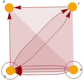
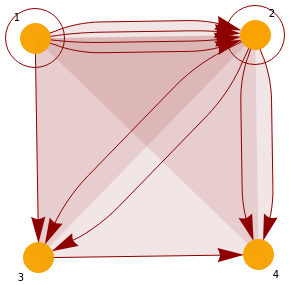
X={a,b,c,d};τ={{},{c},{d},{b,d},{c,d},{b,c,d},{a,b,c,d}};topologicalSpace=FiniteTopologicalSpace[X,τ];elementToOpenSets=AssociationMap[Select[τ,MemberQ[#]]&,X];U=Intersection@@@elementToOpenSets;lessThanQ=topologyRelationCondition[U];partialOrderGraph=HasseDiagram[lessThanQ,X]
Out[]=

We can go the other way, too! Given a partially ordered set we can uniquely create a T0-topological space. Let’s look at just the down arrows in the poset: = {y ∈ X : y ≤ x}. It would be nice if these sets where open sets and could generate the original topology. So let’s show that { : x ∈ X } is a base of open sets that generate a T0-topology. Let x ∈ X and observe that x ∈ . And if x ∈ and x ∈ then we see = {a ∈ X : a ≤ x} ⊆ ∩ because x ≤ y and x ≤ z and transitivity of the relation. The T0 separation is given by the antisymmetric property. We are skipping details, but what this all boils down to is that the topology generated by the basic open sets is a topology is a T0-space.All this proves the following proposition. Proposition 1.4. For a finite set X, the topologies on X are in bijective correspondence with preorders ≤ on X. The topology induced by ≤ as defined above satisfies the T0 separation axiom if and only if ≤ is also antisymmetric.
U
x
U
x
U
x
U
y
U
z
U
x
U
y
U
z
Transform the previous partially ordered set back to the original topological space and assert that they are equivalent.
X=VertexList[partialOrderGraph];basicOpenSets=Insert[Table[[partialOrderGraph,a],{a,X}],{},-1];Assert[BaseQ[basicOpenSets]];generatedTopology=GenerateTopologyFromBase[basicOpenSets];Echo[generatedTopology];Assert[topologicalSpace==generatedTopology]
+
I
»
Points{a,b,c,d},OpenSets{{},{c},{d},{b,d},{c,d},{b,c,d},{a,b,c,d}}
We saw above that if we start with a T0-space and create the associated partially ordered set, then we go backward and turn the poset back to the original topological space, and vice versa. In this sense, we say that finite topological spaces satisfying the T0 separation axiom are equivalent to partially ordered sets. We can map back and forth in a unique way, as shown above. It’s instructive, however, to attempt these transformations but starting with spaces that are not T0. What happens? What goes wrong? This ends up not being a big deal because up to homotopy, we can transform any space into a T0 space. See theorem 4 of McCord for details.
Here’s an example of what can go wrong if space doesn’t satisfy the T0 separation axiom.
X={1,2,3,4};τ={{},{4},{2,4},{3,4},{1,2,3,4}};topologicalSpace=FiniteTopologicalSpace[X,τ];Assert[FiniteTopologicalSpaceQ[topologicalSpace]=={True,True,True}]elementToOpenSets=AssociationMap[Select[τ,MemberQ[#]]&,X];U=Intersection@@@elementToOpenSets;lessThanQ=topologyRelationCondition[U];partialOrderGraph=HasseDiagram[lessThanQ,X]X=VertexList[partialOrderGraph];basicOpenSets=Insert[Table[[partialOrderGraph,a],{a,X}],{},-1];Assert[BaseQ[basicOpenSets]];topologicalSpaceGenerateTopologyFromBase[basicOpenSets]
+
I

Out[]=

Out[]=
Points{1,2,3,4},OpenSets{{},{4},{2,4},{3,4},{1,2,3,4}}
Out[]=
Points{1,2,3,4},OpenSets{{},{4},{2,4},{3,4},{2,3,4},{1,2,3,4}}
With our new notion of space in hand, we now ask the following question: "What does it mean for one space to transform into another space?" Is there a way to define continuity of maps that corresponds to the usual notion of continuous functions we encounter in calculus? The answer to both questions is "YES!". The topological definition of continuity surprisingly generalizes the notion of continuity we are accustomed to and encountered throughout continuous mathematics.
Given two topological spaces we can define function between them. In topology we say a map between two topological spaces f : (X,)->(Y,) is continuous if for every open set A ⊆ , the inverse image (A) = { x ∈ X : f(x) ∈ A } is an open set in .
With this in mind, we could also show that a map f : X → Y is continuous if and only if f preserves order on the corresponding posets.
All together, this correspondence can be stated in the language of category theory as follows: the category P of posets is isomorphic to the category of T0 topological spaces.
With our new notion of space in hand, we now ask the following question: "What does it mean for one space to transform into another space?" Is there a way to define continuity of maps that corresponds to the usual notion of continuous functions we encounter in calculus? The answer to both questions is "YES!". The topological definition of continuity surprisingly generalizes the notion of continuity we are accustomed to and encountered throughout continuous mathematics.
Given two topological spaces we can define function between them. In topology we say a map between two topological spaces f : (X,
τ
1
τ
2
τ
2
-1
f
τ
1
With this in mind, we could also show that a map f : X → Y is continuous if and only if f preserves order on the corresponding posets.
All together, this correspondence can be stated in the language of category theory as follows: the category P of posets is isomorphic to the category of T0 topological spaces.
Causal Set Theory
Causal Set Theory
The reader is now ready to dive into causal set theory in earnest: https://arxiv.org/abs/1903.11544 . Once you’re done with that come back here. I’ll wait. We can create causal sets in Mathematica with code below. Notice that these are partially ordered sets!
Creating a Causal Set
Creating a Causal Set
If you read Sumati Surya’s introduction, then you’ll know that sprinkling provides a good testing ground for recovering properties of continuous. If we start with a manifold where we know a lot of mathematical facts and whose points represent events in space and time, then we want that the finite causal set we get from sampling events on this manifold reflect mathematical structures of the original continuous space.
So a basic question we ask is how fast do open sets in a causal set and flat space converge?
So a basic question we ask is how fast do open sets in a causal set and flat space converge?
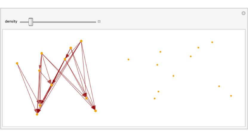
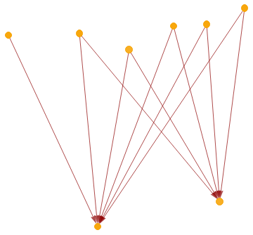
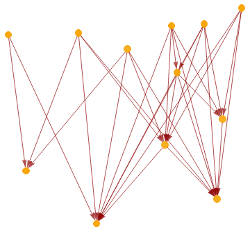
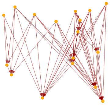
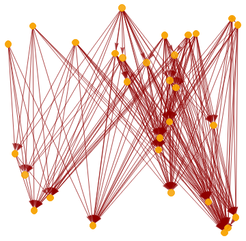
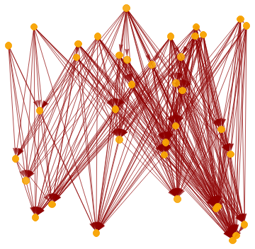
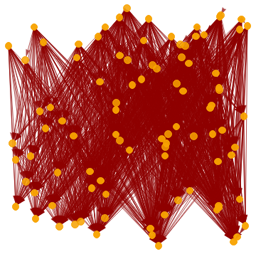
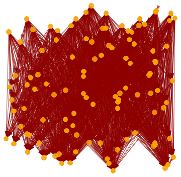
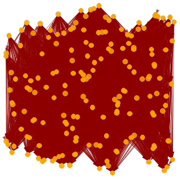
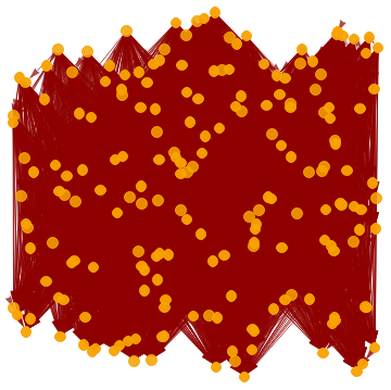
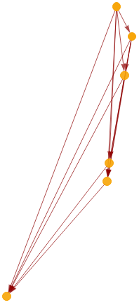
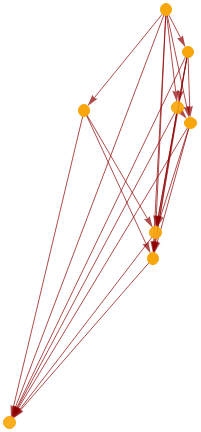
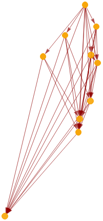
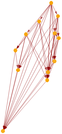
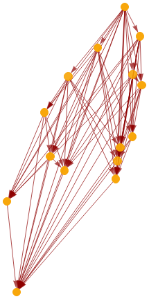
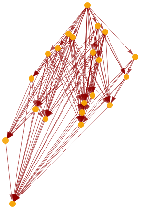
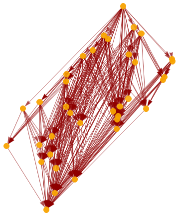
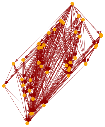
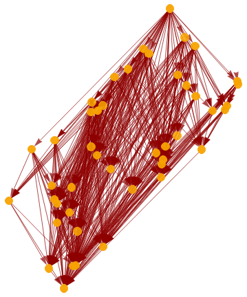
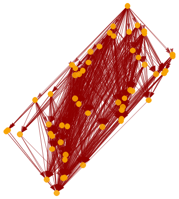
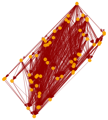
Sample 150 points from a flat Minkowski space and create the corresponding causal set.
In[]:=
{minkowskiNormCompiled,causalFutureQCompiled}=FunctionCompile[{FunctionDeclaration[minkowskiNormCompiled2,Typed[{TypeSpecifier["PackedArray"]["Real64",1]}->"Real64"]@Function[p,p^2.{1,-1}]],Function[{Typed[p,TypeSpecifier["PackedArray"]["Real64",1]],Typed[q,TypeSpecifier["PackedArray"]["Real64",1]]},p[[-1]]<q[[-1]]&&minkowskiNormCompiled2[p-q]<0]},TargetSystem->{"MacOSX-x86-64","Linux-x86-64"}];(*Defineacachetoreusepastresults*)isCausalFuture[x_,y_]:=isCausalFuture[x,y]=causalFutureQCompiled[x,y];PairwiseMinkowskiSerial[points_List]:=With[{pairs=Tuples[points,{2}]},DirectedEdge[#2,#1]&@@@Pick[pairs,isCausalFuture@@@pairs]];createCausalGraph[points_List,edges_List]:=Module[{dimensions},dimensions=Length[First[points]];Graph[points,edges,VertexStyleDirective[Hue[0.11,1,0.97],EdgeForm[{Hue[0.11,1,0.97],Opacity[1]}]],EdgeStyleHue[0,1,0.56],VertexCoordinatesIf[dimensions≤3&&dimensions>1,((##)&/@VertexList[Graph[edges]]),Automatic],GraphLayoutIf[dimensions≤3&&dimensions>1,Automatic,"LayeredDigraphEmbedding"],AspectRatioIf[dimensions≤3&&dimensions>1,Automatic,1/2]]];SpacetimeSprinkling[points_List]["CausalGraphFull2D"]:=Module[{edges},edges=PairwiseMinkowskiSerial[points];createCausalGraph[points,edges]];FlatSpacetimeSprinklingPoints[dimension_Integer,pointsCount_Integer]:=Module[{points},points=RandomReal[1,{pointsCount,dimension}]];PlotCausalSet[causalSet_]:=GraphicsRow[{Show[causalGraph,AxesFalse,Background->White],ListPlot[VertexList[causalGraph],AxesFalse,PlotStyle->{Directive[Hue[0.11,1,0.97]]}]}]
In[]:=
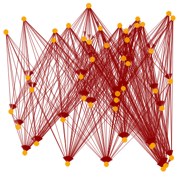
causlSetFiltrationAnim=Manipulate[points=FlatSpacetimeSprinklingPoints[1+1,density];causalGraph=SpacetimeSprinkling[points]["CausalGraphFull2D"];PlotCausalSet[causalGraph],{density,10,20,1}];
frames=Import[Export["causlSetFiltrationAnim.gif",causlSetFiltrationAnim]];ListAnimate[ImageResize[#,1000]&/@frames]
Out[]=
Causal Set Filtration
Causal Set Filtration
+
I
-
I
Definition. A filtration of a topological space X is a sequence of spaces
{
X
n
X
n
X
n+1
⋃
n∈N
X
n
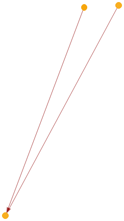
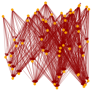
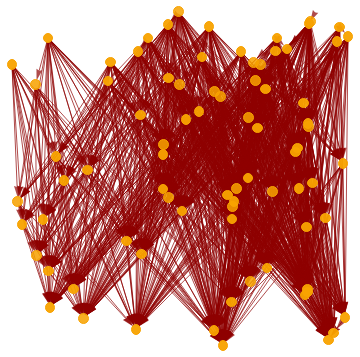
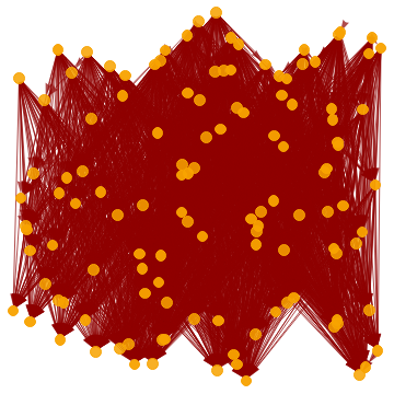
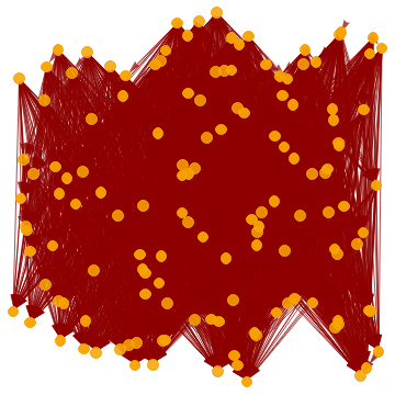
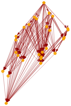
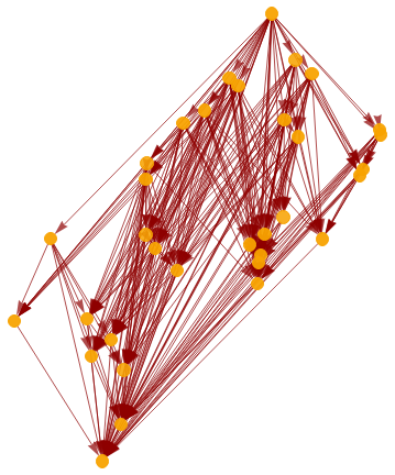
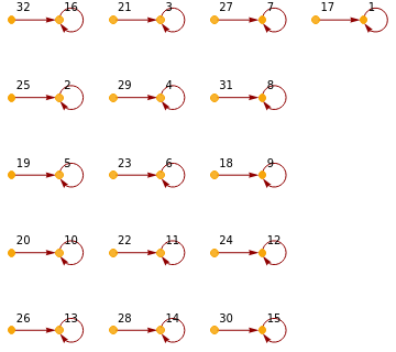
Plot how the causal set grows as we increase the sprinkling density.
In[]:=
AddPoints[perviousPoints_List,dimension_Integer,pointsCount_Integer]:=Module[{newPoints},newPoints=RandomReal[1,{pointsCount,dimension}];Union[perviousPoints,newPoints]];causalSetFilteration[dimension_Integer,sprinklingDensity_Integer,initialSamples_List,curved_List:{}]:=Module[{sprinklingPoints=initialSamples,causalGraph,isCurvedSpace=Length[curved]0},Table[sprinklingPoints=If[isCurvedSpace,AddPoints[sprinklingPoints,dimension,i],{}];causalGraph=SpacetimeSprinkling[sprinklingPoints]["CausalGraphFull2D"];causalGraph,{i,sprinklingDensity}]];(*initiallypickanopensetwewillfollowthegrowth*)GetInitialOpenSet[spaceTimeDimension_,initialSamples_,openSetDefinition_,howManyEdges_:2]:=Module[{sprinklingPointsInitial,causalGraphInitial,vertex1,vertex2,openSet},openSet={};While[Length[openSet]<=howManyEdges,sprinklingPointsInitial=FlatSpacetimeSprinklingPoints[spaceTimeDimension,initialSamples];causalGraphInitial=SpacetimeSprinkling[sprinklingPointsInitial]["CausalGraphFull2D"];vertex1=RandomChoice[VertexList[causalGraphInitial]];vertex2=RandomChoice[VertexOutComponent[causalGraphInitial,vertex1]];openSet=openSetDefinition[causalGraphInitial,vertex1,vertex2]];{vertex1,vertex2,openSet,sprinklingPointsInitial}];
maxSprinklingDensity=19;initialSpacePoints=2;{vertex1,vertex2,openSetInitial,sprinklingPointsInitial}=GetInitialOpenSet[1+1,initialSpacePoints,IntervalBasicOpenSet,1];firstCausalSet=SpacetimeSprinkling[sprinklingPointsInitial]["CausalGraphFull2D"];sprinklingFilteration=causalSetFilteration[1+1,maxSprinklingDensity,sprinklingPointsInitial]PrependTo[sprinklingFilteration,firstCausalSet];openSetsOfFilteration=IntervalBasicOpenSet[#,vertex1,vertex2]&/@sprinklingFilteration;causalDimonds=Map[Subgraph[#[[1]],#[[2]]]&,Transpose[{sprinklingFilteration,openSetsOfFilteration}]];
Out[]=
,
,
,
,
,
,

,
,
,
,
,

,
,
,
,
,
,

,
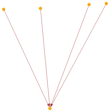
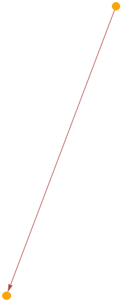
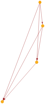
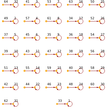
We also plot the filtration of an open set growing within this causal set.
Plot how an open set within the causal set grows.
causalDimonds
Out[]=
,
,
,
,
,
,
,
,
,
,
,

,
,
,
,
,
,
,

,
Metric Spaces Defined by a Causal Set and Minkowski Spacetime
Metric Spaces Defined by a Causal Set and Minkowski Spacetime
To compute a notion of convergence between open sets, we resort to measuring more than just when points are nearby each other. We need a stronger notion of the distance between two points.
Computing Distances within a Causal Set
Computing Distances within a Causal Set
We compute the distance for points that are time-like separated using the estimator from Brightwell and Gregory (1991). This method uses the longest path over all paths between two points as a measure of distance. When points are space-like separated, then the definition of distance is taken from Eichhorn, Surya and Versteegen (2019).
Big thanks to Julia Dannemann-Freitag for providing the initial version of these routines. Any errors introduced by my changes are my fault.
In[]:=
causalMatrix[sortedCoords_List,edgeList_,pointNumber_]:=Module[{CGRules,indexEdges,prematrix},CGRules=sortedCoords[[#]]Range[Length@sortedCoords][[#]]&/@Range[Length@sortedCoords];indexEdges=edgeList/.CGRules;prematrix=Table[{indexEdges[[n,1]],indexEdges[[n,2]]},{n,1,Length@indexEdges}];SparseArray[prematrix[[#]]1&/@Range[Length@prematrix],{pointNumber,pointNumber}]](*GivesalistofallpointsNlinksinthepastofagivenstartingpoint*)layerPastN[linkMatrixTransposed_,x_,n_Integer]:=Flatten[Position[(MatrixPower[linkMatrixTransposed,n])[[x]],_?Positive]]volumeOfVertices[caugraph_,linkMatrixTransposed_,vertexlist_,x_,y_]:=Module[{linkDistance1,linkDistance2,volume1,volume2},Table[linkDistance1=GraphDistance[caugraph,x,vertex];linkDistance2=GraphDistance[caugraph,y,vertex];volume1=Length[DeleteDuplicates[Flatten[layerPastN[linkMatrixTransposed,vertex,#]&/@Range[linkDistance1]]]];volume2=Length[DeleteDuplicates[Flatten[layerPastN[linkMatrixTransposed,vertex,#]&/@Range[linkDistance2]]]];volume1+volume2,{vertex,vertexlist}]] (*Givesthepointvolumeofthetriangleformedbytwospacelikepointsandthepointwheretheirlightconesintersect*)spaceVolume[linkmatrix_,causalmatrixTransposed_,caugraph_,x_,y_]:=Module[{slice1,slice2,posvertexList,caufollow,vertexlist,linkMatrixTransposed,totalVolume},linkMatrixTransposed=Transpose[Normal[linkmatrix]];slice1=Select[causalmatrixTransposed,(#[[x]]*#[[y]])==1&];posvertexList=Flatten[Position[causalmatrixTransposed,slice1[[#]]]&/@Range[Length[slice1]]];caufollow=DeleteDuplicates[Flatten[Table[Select[causalmatrixTransposed,#[[n]]==1&],{n,posvertexList}],1]];slice2=Select[slice1,!MemberQ[caufollow,#]&];vertexlist=DeleteDuplicates[Flatten[Position[causalmatrixTransposed,slice2[[#]]]&/@Range[Length[slice2]]]];totalVolume=volumeOfVertices[caugraph,linkMatrixTransposed,vertexlist,x,y];Min[totalVolume]/2.0](*Calculatesthespacelikedistanceoftwospacelikepointsusingtheabovefunctions*)spaceDistance2D[linkmatrix_,causalmatrixTransposed_,caugraph_,x_,y_,density_]:=Module[{volume},volume=spaceVolume[linkmatrix,causalmatrixTransposed,caugraph,x,y];2*Sqrt[volume/density]]createCausalMatrices[causalMatrix_]:=Module[{linkmatrix,causalmatrixTransposed,reducedCausalGraph},reducedCausalGraph=TransitiveReductionGraph[AdjacencyGraph[causalMatrix]];linkmatrix=AdjacencyMatrix[reducedCausalGraph];causalmatrixTransposed=Transpose[Normal[causalMatrix]];{linkmatrix,causalmatrixTransposed,reducedCausalGraph}](*Calculatesthetimelike/spacelikedistanceofeachpairofpointsonaCausalSetusingtheabovefunctionsandlengthoflongestchainmethodfortimelikedistance*)spaceTimeDistance2D[causalmatrix_,density_]:=Module[{pointNumber,lChainMatrix,DistanceMatrix,spacelikePairs,distanceMatrix,linkmatrix,causalmatrixTransposed,caugraph},{linkmatrix,causalmatrixTransposed,caugraph}=createCausalMatrices[causalmatrix];pointNumber=Length[linkmatrix];lChainMatrix=Total[UnitStep[NestWhileList[#.causalmatrix&,causalmatrix,#≠ConstantArray[0,{pointNumber,pointNumber}]&]-0.1]];DistanceMatrix=N[lChainMatrix/(2*Sqrt[(density/2)])];spacelikePairs=Select[Position[Normal[lChainMatrix],0,2],#[[1]]<#[[2]]&];(DistanceMatrix[[spacelikePairs[[#,1]],spacelikePairs[[#,2]]]]=spaceDistance2D[linkmatrix,causalmatrixTransposed,caugraph,spacelikePairs[[#,1]],spacelikePairs[[#,2]],density])&/@Range[Length[spacelikePairs]];DistanceMatrix]spaceTimeDistance2D[causalmatrix_,density_,pointsInOpenset_]:=Module[{pointNumber,lChainMatrix,DistanceMatrix,spacelikePairs,distanceMatrix,linkmatrix,causalmatrixTransposed,caugraph},{linkmatrix,causalmatrixTransposed,caugraph}=createCausalMatrices[causalmatrix];pointNumber=Length[linkmatrix];lChainMatrix=Total[UnitStep[NestWhileList[#.causalmatrix&,causalmatrix,#≠ConstantArray[0,{pointNumber,pointNumber}]&]-0.1]];DistanceMatrix=N[lChainMatrix/(2*Sqrt[(density/2)])];spacelikePairs=Select[Position[Normal[lChainMatrix],0,2],(pointsInOpenset[{#[[1]]}]&&pointsInOpenset[{#[[2]]}]&&#[[1]]<#[[2]])&];(DistanceMatrix[[spacelikePairs[[#,1]],spacelikePairs[[#,2]]]]=spaceDistance2D[linkmatrix,causalmatrixTransposed,caugraph,spacelikePairs[[#,1]],spacelikePairs[[#,2]],density])&/@Range[Length[spacelikePairs]];DistanceMatrix]
Computing Distances within Minkowski Spacetime
Computing Distances within Minkowski Spacetime
Computing a distance between two events in flat spacetime is not nearly as hard as it for causal sets. Le u₁ = , , , ) and u₂ = , , , ) be events in 4D dimensional space time. Then we define the scalar product as η (u₁,u₂)= u₁⋅ u₂ = c²t₁t₂−x₁x₂− y₁ y₂− z₁ z₂. So the norm =. The induced metric is . Code for computing this in 2 dimensional flat space time below.
(
t
1
x
1
y
1
z
1
(
t
2
x
2
y
2
z
2
||u||
c²t₁t₂−x₁x₂−y₁y₂−z₁z₂
||-||=---
u
1
u
2
2
(t₁-)
t
2
2
(-)
x
1
x
2
2
(-)
y
1
y
2
2
(-)
z
1
z
2
In[]:=
minkowskiNorm[point_List]:=(point^2).{1,-1}minkowskiDistance[point1_,point2_]:=minkowskiNorm[point1-point2];
These two notions of distance allow us to turn the collection of points into a metric space denoted (M,d). M is the underlying set, like or a poset, and d is the metric. We explicitly represent a metric space with finite points by computing the distance matrix, whose rows and columns tells us the distance between any pair of points
2
R
Metric Between Metric Spaces
Metric Between Metric Spaces
In the previous section, we described metrics associated with Minkowski spacetime and a causal set. We would like to measure the distance between subsets of one metric with subsets of another metric space. This desire for a metric of metric spaces gives rise to what is called the Hausdorff-Gromov Distance. Although, it appears to have first been discovered by David A. Edwards when investigating the configuration space of general relativity proposed by John Wheeler.
Hausdorff
Hausdorff
Before describing how we compare things defined using two different metric spaces, let’s first see how we compare two subsets within a shared metric space. The idea is that we want to measure how far away is a point in A is the farthest from B, and the other way around, and we return the larger of these extremes. Definition. Let X and Y be two non-empty subsets of a metric space (M,d). We define the Hausdorff distance (X,Y) as the max d(x,Y), d(X,y)} where d(a,b)
d
H
{
sup
x∈X
sup
y∈Y
d(a,B)=
inf
b∈B
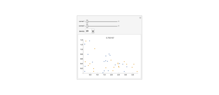
In this example, we compare two triangles in Euclidean space using Hausdorff distance. Notice that as the triangles align, their distance decreases.
In[]:=
HausdorffDistance[setOne__,setTwo_,distanceFunction_]:=Module[{closest1,closest2},closest1=FeatureNearest[setOne"Distance",setTwo,1,DistanceFunctiondistanceFunction];closest2=FeatureNearest[setTwo"Distance",setOne,1,DistanceFunctiondistanceFunction];Max[Max[closest1],Max[closest2]]];
In[]:=
hausdorffDistanceAnim=Manipulate[=Triangle[{{0,0},{corner1,0},{0,corner2}}];ℬ=Triangle[{{0,0},{5,0},{0,3/2}}];subset1=RandomPoint[,density];subset2=RandomPoint[ℬ,density];distance=HausdorffDistance[subset1,subset2,EuclideanDistance];ListPlot[{subset1,subset2},PlotLabeldistance],{corner1,5,1,-1},{corner2,3/2,.01,-0.1},{density,{20,50,100,200,300,400,500,600}}];
frames=Import[Export["hausdorffDistanceAnim.gif",hausdorffDistanceAnim]];ListAnimate[ImageResize[#,1000]&/@frames]
Out[]=
Hausdorff-Gromov
Hausdorff-Gromov
What happens when we have two metric spaces? Say and The idea is to map both metric spaces into a common metric space and use the Hausdorff distance. In general, to compute this metric, we search over all possible metrics spaces and ways to map X and Y into M. The maps under consideration are restricted to be those that persevere distances. We (x, y) = (f(x), f(y)). Definition. Given a metric space , a map of f : → is called an isometric embedding if for all , ∈ : (, ) = (f(), f()). Definition. The Gromov-Hausdorff distance between two metric space and is (X, Y ) = (i(X), j(Y )).There is an alternative characterization of the Hausdorff-Gromov metric that easier to compute in practice when dealing with finite spaces (http://sites.fas.harvard.edu/~cs277/papers/gromov.pdf )Definition. We define a correspondence from to as a set R ⊆ X × Y such that following conditions hold. First, for all x ∈ X, there exists y ∈ Y such that (x, y) ∈ C . Second, for all y ∈ Y, there exists x ∈ X such that (x, y) ∈ C. We use Π(X, Y) to denote the set of all correspondences between X and Y. being represented by a distance matrix, a correspondence is just a permutation of (row, column) pairs. We can measure the discrepancy introduced by a correspondence by computing its distortion. Definition. Let , ) and , ) be two metric spaces. The distortion of a correspondence , ) is defined as Dist(C) = | (x, ) − (y, )|. Definition.The Gromov-Hausdorff distance , between and is defined as: (X, Y) = Dist(C).Fortunately, we can make this computationally tractable because by construction we know which points in the causal set correspond to points in the manifold. This allows us to simplify significantly the Gromov-Hausdorff distance.
(X,)
d
1
(Y,).
d
2
(M,)
d
M
onlywantmapsf:(X,)->(M,)ensuringthat
d
1
d
M
d
1
d
M
(X,)
d
1
(X,)
d
1
(M,)
d
M
x
1
x
2
(X,)
d
1
d
X
x
1
x
2
d
M
x
1
x
2
(X,)
d
1
(Y,)
d
2
d
GH
inf
i:X→Z,j:Y→Z
d
H
(X,)
d
1
(Y,)
d
2
Whenweconsider(X,)
d
1
(
X
1
d
1
(
X
2
d
2
C∈Π(
X
1
X
2
sup
(x,y),,∈C
x
y
d
1
x
d
2
y
d
GH
(X,)
d
1
(Y,)
d
2
d
GH
1
2
inf
C∈Π(X1,X2)
In[]:=
GromovHausdorfDistance[causalSetMetricSpace_,minkowskiMetricSpace_]:=Max[Abs[causalSetMetricSpace-minkowskiMetricSpace]]GromovHausdorfDistance[causalSetMetricSpace_,minkowskiMetricSpace_,openSetIndicies_List]:=Module[{causalOpenSetMetricSpace,minkowskiOpenSetMetricSpace,gromovHausdorfDistance},causalOpenSetMetricSpace=causalSetMetricSpace[[openSetIndicies,openSetIndicies]];minkowskiOpenSetMetricSpace=minkowskiMetricSpace[[openSetIndicies,openSetIndicies]];gromovHausdorfDistance=GromovHausdorfDistance[causalOpenSetMetricSpace,minkowskiOpenSetMetricSpace]]
Computing Hausdorff-Gromov Distance Between Causal Sets and Minkowski Spacetime
Computing Hausdorff-Gromov Distance Between Causal Sets and Minkowski Spacetime
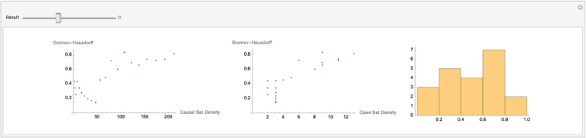
We now try to figure how fast open sets in the causal set converge to open sets of the flat manifold. Using the code above, we ran several experiments with increasing sprinkling density. We saved the results of these experiments in the notebook, and you can explore the results below. While we observe evidence that the distances between the metric spaces tend to a definite value when in cases where the open set grows at a steady rate, more experiments and thought is required to characterize the limiting value and its rate of convergence.
The code below was used to gather data to see how the distance between open sets converged
In[]:=
vertexListSorted[graph_]:=SortBy[VertexList[graph],Minus@*Last]createMetricSpacesFromFilteration[growth_]:=Module[{orderedVertices,edges,totalVertices,caumat,linkmat,causalSetMetricSpace,estimatedManifoldMetricSpaces},ParallelTable[orderedVertices=vertexListSorted[causalGraph];edges=EdgeList[causalGraph];totalVertices=Length[orderedVertices];caumat=causalMatrix[orderedVertices,edges,totalVertices];causalSetMetricSpace=spaceTimeDistance2D[caumat,totalVertices];estimatedManifoldMetricSpaces=UpperTriangularize[DistanceMatrix[orderedVertices,DistanceFunctionminkowskiDistance]];{orderedVertices,causalSetMetricSpace,estimatedManifoldMetricSpaces},{causalGraph,growth}]]createMetricSpacesFromFilteration[growth_,openSetsOfFilteration_]:=Module[{orderedVertices,edges,totalVertices,caumat,linkmat,causalSetMetricSpace,estimatedManifoldMetricSpaces,verticesOfOpenset,pointsToKeep,total=Length[growth],openSetOfFilteration,causalGraph},ParallelTable[causalGraph=growth[[i]];openSetOfFilteration=openSetsOfFilteration[[i]];orderedVertices=vertexListSorted[causalGraph];edges=EdgeList[causalGraph];totalVertices=Length[orderedVertices];verticesOfOpenset=SubsetPosition[orderedVertices,{#}][[1]][[1]]&/@openSetOfFilteration;pointsToKeep=ContainsAny[verticesOfOpenset];caumat=causalMatrix[orderedVertices,edges,totalVertices];causalSetMetricSpace=spaceTimeDistance2D[caumat,totalVertices,pointsToKeep];estimatedManifoldMetricSpaces=UpperTriangularize[DistanceMatrix[orderedVertices,DistanceFunctionminkowskiDistance]];{orderedVertices,causalSetMetricSpace,estimatedManifoldMetricSpaces},{i,total}]]ComputeConvergence[spaceTimeDimension_,initialSpacePoints_,maxSprinklingDensity_]:=Module[{filtrationLength=maxSprinklingDensity+1,vertex1,vertex2,openSetInitial,sprinklingPointsInitial,firstCausalSet,sprinklingFilteration,openSetsOfFilteration,isGrowing,orderedPoints,causalSetMetricSpaces,minkowskiMetricSpaces,merged,openSetIndicies,sizeOfOpenSets,distances},{vertex1,vertex2,openSetInitial,sprinklingPointsInitial}=GetInitialOpenSet[spaceTimeDimension,initialSpacePoints,IntervalBasicOpenSet,1];firstCausalSet=SpacetimeSprinkling[sprinklingPointsInitial]["CausalGraphFull2D"];sprinklingFilteration=causalSetFilteration[spaceTimeDimension,maxSprinklingDensity,sprinklingPointsInitial];PrependTo[sprinklingFilteration,firstCausalSet];openSetsOfFilteration=IntervalBasicOpenSet[#,vertex1,vertex2]&/@sprinklingFilteration;sizeOfOpenSets=Length/@openSetsOfFilteration;isGrowing=!Commonest[sizeOfOpenSets]=={2};distances=If[isGrowing,{orderedPoints,causalSetMetricSpaces,minkowskiMetricSpaces}=Transpose[createMetricSpacesFromFilteration[sprinklingFilteration,openSetsOfFilteration]];merged=Transpose[{orderedPoints,openSetsOfFilteration}][[1;;filtrationLength]];openSetIndicies=Sort[(SubsetPosition[#[[1]],#[[2]]])[[1]]]&/@merged;distances=ParallelTable[GromovHausdorfDistance[causalSetMetricSpaces[[i]],minkowskiMetricSpaces[[i]],openSetIndicies[[i]]],{i,filtrationLength}],{}];{distances,VertexCount/@sprinklingFilteration,sizeOfOpenSets}]
Run 3 trails using 1+1 space time and growing the set to a maximum of 8 (8+1) / 2 points
In[]:=
results=Table[ComputeConvergence[1+1,2,8],{i,3}];
Here we precomputed several results running various experiments with different sprinkling densities. Experiments 3 and 4 have the most points and provide evidence for convergence.
PopupMenu[Dynamic[experiment],{resultsFromExperiments[[1]]->"Experiment 1",resultsFromExperiments[[2]]->"Experiment 2",resultsFromExperiments[[3]]->"Experiment 3",resultsFromExperiments[[4]]->"Experiment 4"}]resultsAnim=Manipulate[{distance,causalSetSize,openSetSize}=Dynamic[experiment][[1]];total=Length[distance];GHCausalSet=ListPlot[Transpose[{causalSetSize[[i]],distance[[i]]}],AxesLabel->{"Causal Set Density","Gromov-Hausdorff"}];GHOpenSet=ListPlot[Transpose[{openSetSize[[i]],distance[[i]]}],AxesLabel->{"Open Set Density","Gromov-Hausdorff"}];distanceHist=Histogram[distance[[i]]];GraphicsRow[{GHCausalSet,GHOpenSet,distanceHist},BackgroundWhite,ImageSize{1200,200}],{{i,1,"Result"},1,total,1}];
Out[]=
frames=Import[Export["resultsAnim.gif",resultsAnim]];ListAnimate[ImageResize[#,1000]&/@frames]
Out[]=
Space of Spaces and Set-Theoretic Limits
Space of Spaces and Set-Theoretic Limits
We have considered topological spaces in isolation. We now go one step further by considering the space of all topological spaces over a fixed set. This space is also a lattice. With the following partial order: <= is defined to mean that every open set in is also open in . We say that is coarser than than while is said to be finer because it has more open sets than . We could also define a meet and a join.
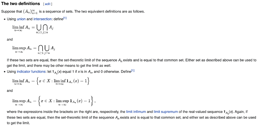
Using this lattice, we can define a topological notion of convergence. This construction, however, assumes that the numbers elements is fixed. In practice, we know that this assumption is not true since the world is constantly evolving. With this in mind, we could try to generalize by considering the category of all partially ordered sets or equivalently the category of T0 topological spaces. We could also consider set limits like those encountered in measure theory: https://en.wikipedia.org/wiki/Set-theoretic_limit
τ
1
τ
2
τ
1
τ
2
τ
1
τ
2
τ
2
τ
1
Using this lattice, we can define a topological notion of convergence. This construction, however, assumes that the numbers elements is fixed. In practice, we know that this assumption is not true since the world is constantly evolving. With this in mind, we could try to generalize by considering the category of all partially ordered sets or equivalently the category of T0 topological spaces. We could also consider set limits like those encountered in measure theory: https://en.wikipedia.org/wiki/Set-theoretic_limit
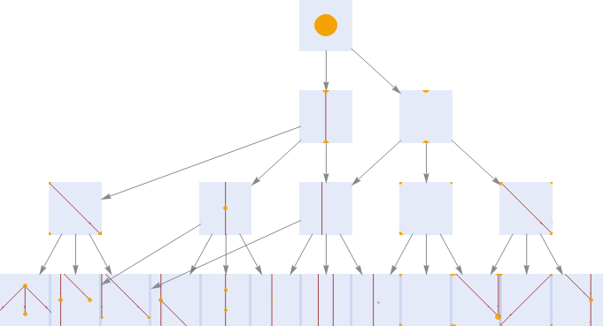
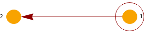
One way to display the first few elements of this category using the following multiway system.
Explicitly generate a small part of the category of posets
stripMetadata[expression_]:=expression/;Head[expression]=!=RulestripMetadata[expression_]:=Last[expression]/;Head[expression]===RuleCausalMultiwaySystem[stepCount_Integer,options:OptionsPattern[]]:=CausalMultiwaySystem[stepCount,"StatesGraph",options]CausalMultiwaySystem[stepCount_Integer,property_String,options:OptionsPattern[]]:=ResourceFunction["MultiwaySystem"]["WolframModel"{{{0}}{{0,1}},{{0}}{{0},{1}},{{0,1}}{{0,1},{1,2}},{{0,1}}{{0,1},{0,2}},{{0,1}}{{0,1},{2}},{{0},{1}}{{0,2},{1,2}}},{{{0}}},stepCount,If[property==="CausalGraph","CausalGraphStructure",property],VertexSizeIf[property=!="CausalGraph",1,Automatic],"StateRenderingFunction"(Inset[Framed[Style[LayeredGraphPlot[Graph[DeleteDuplicates[Flatten[stripMetadata[#2]]],Select[(DirectedEdge@@@stripMetadata[#2]),Length[#]2&],VertexSize0.1],VertexStyleDirective[Hue[0.11,1,0.96],EdgeForm[{Hue[0.11,1,0.97],Opacity[1]}]],EdgeStyleHue[0,1,0.56],EdgeShapeFunctionGraphElementData["ShortFilledArrow","ArrowSize"0.05],ImagePaddingAutomatic],Hue[0.62,1,0.48]],BackgroundDirective[Opacity[0.2],Hue[0.62,0.45,0.87]],FrameMargins{{2,2},{0,0}},RoundingRadius0,FrameStyleDirective[Opacity[0.5],Hue[0.62,0.52,0.82]]],#1,{0,0},#3]&),options]categoryOfPosets=CausalMultiwaySystem[3];LayeredGraphPlot[categoryOfPosets,AspectRatio1/2,VertexSize2]
Out[]=
Concluding Remarks
Concluding Remarks
I hope the reader benefited from this chronically of my three weeks at the Wolfram Summer school. We gave an interactive introduction to topology and causal set theory and showed how to use Mathematica to investigate these subjects. We provide some numerical evidence to investigate the rate of convergence between between open sets within a causal set and those in flat spacetime limit to a definite value without going to infinity. More tests, thought, thoroughness is required to stay anything definite here. While this brings an end to our run-in with causal sets, I would be remiss, however, if I did not make some remarks concerning the Wolfram Physics project proper.
Relation to Wolfram Physics Formalism
Relation to Wolfram Physics Formalism
A core component of the Wolfram physics project is applying hypergraph rewrite rules to generate spatial structures which contain a surprisingly rich amount of ideas from modern physics and theoretical computer science. Readers interested in the details are encouraged to learn more at https://www.wolframphysics.org/technical-introduction/.
Definition: A hypergraph is pair H = (V,E) where V is a set of elements called nodes or vertices, and E is a collection of subsets of the powerset of X.
This is unsurprisingly a very general object, and so I expected studying them to be too computationally expensive and too difficult. One of the first things I learned from the Wolfram physics project is the extent to which it is possible to recover meaningful structure related to mathematical physics. We also don’t have to go far to touch the topological ideas we already encountered.
The first thing to notice is that every finite topological space, (X, τ), is a particular case of a hypergraph. The edges are open sets in τ, and vertices are elements of the space, X: (V, E) = (X, τ). This immediately gives us another way to visualize topological space as we can use the existing tools developed for the Physics project to get a new perspective.
Visualize topological spaces using Wolfram model plotting
PlotWolframModel[states_]:=ResourceFunction["WolframModelPlot"][states,VertexLabels"Name",VertexStyleDirective[Hue[0.11,1,0.97],EdgeForm[{Hue[0.11,1,0.97],Opacity[1]}]],EdgeStyleHue[0,1,0.56]]X={a,b,c,d};τ={{a,b,c,d},{a,b,c},{a,b,d},{a,b},{a},{b}};topology=FiniteTopologicalSpace[X,Insert[τ,{},-1]];Assert[FiniteTopologicalSpaceQ[topology]=={True,True,True}];PlotWolframModel[τ]
Out[]=
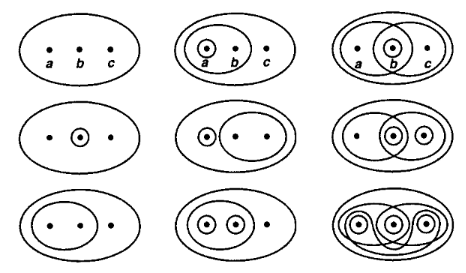
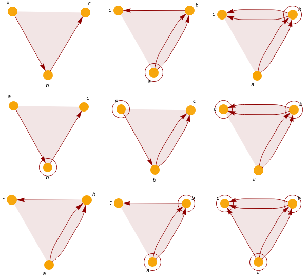
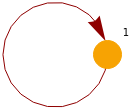
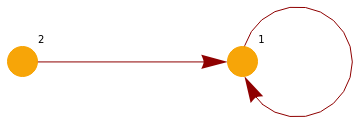
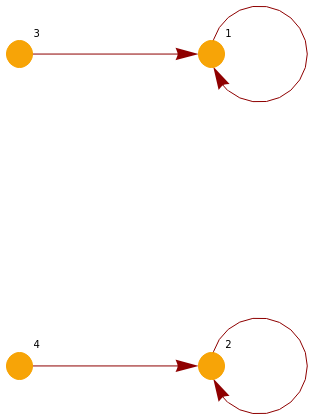
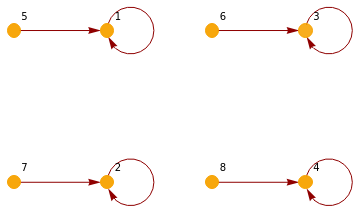
Reproduce a page from Munkres’ classic topology textbook from 1975. Ordering matters within Wolfram Model rules since they directed hypergraphs. We can fix this by simply adding multiple subsets in different order to mimic a true set.
τ
1
τ
2
τ
3
τ
4
τ
5
τ
6
τ
7
τ
8
τ
9
τ
1
τ
4
τ
7
τ
2
τ
5
τ
8
τ
3
τ
6
τ
9
Out[]=
Out[]=
We also notice that some rules evolve a valid topological base to another topological base. This shows a future possibility where we study the topological dynamics of these rules. Going one step further, one could ask about the existence of rules that naturally generate valid topological spaces at each step.
states=[{{{1,2}}->{{1,1},{3,1}}},{{1,1}},6,"StatesList"];PlotWolframModel/@statesEcho[BaseQ/@states];PlotWolframModel[DeleteCases[GenerateTopologyFromBase[#]["OpenSets"],{}]]&/@states[[1;;4]]
Out[]=
,
,
,
,
,
,
»
{True,True,True,True,True,True,True}
Out[]=
,
,
,
We can also more formally express some ideas used in the Wolfram Physics project. One example is foliation. Given a causal graph P and a rank function ρ : P → N define an equivalence relation ∼ on P where p∼q whenever p and q belong to the same “level set” (n) for some n in natural numbers. The branchial space is the quotient space P /∼ endowed with the quotient topology. A branchial graph is an element of the branchial space.
There are many more possibilities, but I have run out of time and getting pulled off stage. I imagine at this point I’m shouting: “Sigma algebra! Homotopy theory! Sheaf Cohomology! Grothendieck topology! Geometrodynamics!!” Much more left to do.
Thanks for listening. Please reach out at https://twitter.com/learnerofmath .
Take Care,
Rafael
-1
ρ
There are many more possibilities, but I have run out of time and getting pulled off stage. I imagine at this point I’m shouting: “Sigma algebra! Homotopy theory! Sheaf Cohomology! Grothendieck topology! Geometrodynamics!!” Much more left to do.
Thanks for listening. Please reach out at https://twitter.com/learnerofmath .
Take Care,
Rafael
Keywords
Keywords
◼
Finite Topological Spaces
◼
Topology
◼
Causal Set Theory
◼
Physics
◼
Quantum Gravity
◼
Education
◼
Mathematics
Acknowledgment
Acknowledgment
Major thanks to Julia for sharing her original causal set distance computations and helping me understand causal set theory. This project would have also not been possible without the help of Mano, Jonathan, Xerxes. Every time we spoke I had better understanding of things and I really appreciate the time we spent together. The TAs of the summer program were all amazing. In particular, Jesse, Daniel, Nick, and Carlos were instrumental in speeding up the causal set computations and helping me learn the programming language. Finally, thank you to Dr. Wolfram for providing me the opportunity to learn more about physics and its relation to computation and mathematics.
References
References
◼
Munkers, J. R. (1975). Topology: A first course. Prentice-Hall.
◼
May, J. P. (2016). Finite spaces and larger contexts. Unpublished book.
◼
McCord, M. C. (1966). Singular homology groups and homotopy groups of finite topological spaces. Duke Mathematical Journal, 33(3), 465-474.
◼
Stong, R. E. (1966). Finite topological spaces. Transactions of the American Mathematical Society, 123(2), 325-340.
◼
Gorard, J. (2020). Algorithmic Causal Sets and the Wolfram Model. arXiv preprint arXiv:2011.12174.
◼
Mémoli, F. (2007). On the use of Gromov-Hausdorff distances for shape comparison.
◼
Brightwell, G., & Gregory, R. (1991). Structure of random discrete spacetime. Physical review letters, 66(3), 260.
◼
Eichhorn, A., Surya, S., & Versteegen, F. (2019). Induced spatial geometry from causal structure. Classical and Quantum Gravity, 36(10), 105005.