The Wolfram Quantum Computation Framework performs high-level analytic and numeric computations in Quantum Information Theory, allowing simulation of quantum circuits and quantum algorithms. Starting from discrete quantum mechanics, this framework can work with quantum states and quantum operators, implements measurements, performs basis manipulation, computes measure entanglement, and more. In this short computational essay, I explore quantum circuit counterparts of some interesting quantum experiments (e.g., quantum eraser, Elitzur-Vaidman bomb etc).
Wolfram Quantum Computation Framework
Wolfram Quantum Computation Framework
You can find the Wolfram QuantumFramework here: Wolfram Quantum Computation Framework.
Stephen Wolfram also briefly introduced this framework during his keynote speech at the Wolfram Tech Conference 2021: YouTube link of Stephen's Talk.
It is a paclet, containing a collection of functions for quantum computation. If you have Wolfram Mathematica V.13 or more, you can simple copy codes from above link and paste it into a Wolfram notebook. For versions 12.3 and more, you can install the paclet as follows:
PacletUninstall/@PacletFind["Quantum*"];ClearAll["Wolfram`QuantumFramework`*","Wolfram`QuantumFramework`**`*"];PacletInstall[CloudObject@URLExpand@"https://wolfr.am/ZcOPnVar",ForceVersionInstall->True]<<Wolfram`QuantumFramework`
Please note that the detailed documentation can be found in the above link, too. We highly recommend our users to explore this framework and simulate a quantum computer using the Wolfram Language. There are many examples and quantum circuits that you can find the paclet webpage.
In the following, I will explore some important experiments in the foundation of quantum theory as showcases. These experiments were also discussed in a recent arXiv preprint.
Quantum Eraser
Quantum Eraser
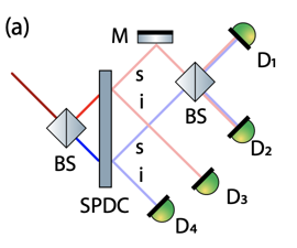
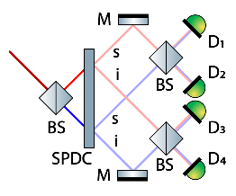
In short, if there is path information (stored somewhere, regardless of if it is measured or not), there won’t be any interference. The mere presence of path info will kill the quantum interference. By erasing the path info, one can recover the quantum interference. In the following setup, clicking all detectors corresponds to no interference case, and clicking of only D1 and D4 corresponds to the interference.
With path information: no interference
With path information: no interference
In[]:=
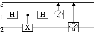
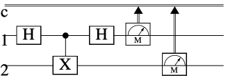
A series of quantum gates representing above setup:
In[]:=
ops={QuantumOperator["H"],QuantumOperator["CX"],QuantumOperator["H"],QuantumMeasurementOperator[],QuantumMeasurementOperator[{2}]};
Construct the quantum circuit:
In[]:=
qc=QuantumCircuitOperator[ops];qc["Diagram"]
Out[]=
Calculate the system evolution through each steps
In[]:=
steps=ComposeList[ops,QuantumState[{"Register",2}]];
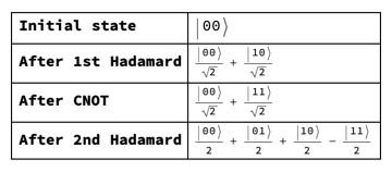
Show the states before measurements:
In[]:=
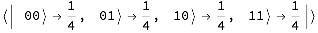
Grid[Transpose[{Style[#,Bold]&/@{"Initial state","After 1st Hadamard","After CNOT","After 2nd Hadamard"},#["Formula"]&/@steps[[;;-3]]}],Frame->All,AlignmentLeft]
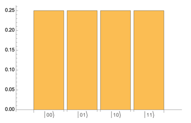
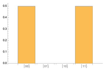
Probability results given the outcomes:
In[]:=
qc[QuantumState[{"Register",2}]]["ProbabilityPlot"]
Erasing path information: interference
Erasing path information: interference
In[]:=
A series of quantum gates representing above setup:
In[]:=
ops={QuantumOperator["H"],QuantumOperator["CX"],QuantumOperator["H"],QuantumOperator["H",{2}],QuantumMeasurementOperator[],QuantumMeasurementOperator[{2}]};
Construct the quantum circuit:
In[]:=
qc=QuantumCircuitOperator[ops];qc["Diagram"]
Out[]=
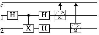
Note that the Hadamard gate acting on 2nd qubit serves as quantum eraser.
Calculate the system evolution through each steps
In[]:=
steps=ComposeList[ops,QuantumState[{"Register",2}]];
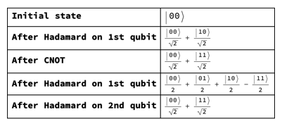
Show the states before measurements:
In[]:=
Grid[Transpose[{Style[#,Bold]&/@{"Initial state","After Hadamard on 1st qubit","After CNOT","After Hadamard on 1st qubit","After Hadamard on 2nd qubit"},#["Formula"]&/@steps[[;;-3]]}],Frame->All,AlignmentLeft]
Probability results given the outcomes:
In[]:=
qc[QuantumState[{"Register",2}]]["ProbabilityPlot"]
Elitzur-Vaidman bomb
Elitzur-Vaidman bomb
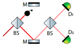
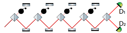
Given the quantum interference, in a Mach-Zehnder setup with only one beam-splitter, one can end up with a situation that a detector click can be inferred as presence of an object along one arm of interferometer. However, due to the interference, there is a 50% chance that the photon did not path that arm, as if one can infer the presence of that object without any interaction. To dramatize the case, think about that object as a bomb! That is why sometimes this thought experiment is also called as the interaction-free measurement.
Simple case: 50:50 beam splitter
Simple case: 50:50 beam splitter
A series of quantum gates representing above setup:
In[]:=
ops={QuantumOperator["H"],QuantumOperator["CX"],QuantumOperator["H"],QuantumMeasurementOperator[],QuantumMeasurementOperator[{2}]};
Construct the quantum circuit:
In[]:=
qc=QuantumCircuitOperator[ops];qc["Diagram"]
Out[]=
Probability results given the outcomes:
In[]:=
prob=qc[QuantumState[{"Register",2}]]["Probabilities"]
Out[]=
Note that detecting or means bomb is explored (i.e., interaction with bomb, or photon passed through the arm where the bomb is), while means that with the help of quantum interference, the bomb is detected with no interaction. Therefore, the efficiency rate η can be expressed as
|01〉
|11〉
|00〉
η=/(++)=/(1-)
P
00
P
00
P
01
P
11
P
00
P
10
In[]:=
prob[|00〉]/(1-prob[|10〉])
Out[]=
Beyond 50:50 beam splitter using Ry(θ)
Beyond 50:50 beam splitter using (θ)
R
y
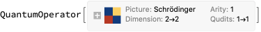
The Hadamard gate acts like a 50:50 beam splitter. One can replace it with (θ) which is rotation along y-axis with an arbitrary angle θ as follows:
R
y
In[]:=
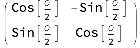
QuantumOperator[{"YRotation",θ}]%["Matrix"]//MatrixForm
Out[]=
Out[]//MatrixForm=
For example, let’s compare the Hadamard gate with (θ) gate on the quantum state :
R
y
|0〉
In[]:=
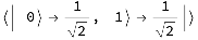
QuantumOperator["H"][QuantumState[{1,0}]]["Amplitudes"]
Out[]=
In[]:=
QuantumOperator[{"YRotation",θ}][QuantumState[{1,0}]]["Amplitudes"]
Out[]=
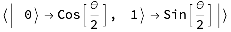
Note that the reflection will turn the qubit to , meaning it will be in the arm where the bomb is located (look at above figure).
|1〉
Define new quantum circuit using (θ):
R
y
In[]:=
qc=QuantumCircuitOperator[{QuantumOperator[{"YRotation",θ}],QuantumOperator["CX"],QuantumOperator[{"YRotation",θ}],QuantumMeasurementOperator[],QuantumMeasurementOperator[{2}]}];qc["Diagram"]
Out[]=
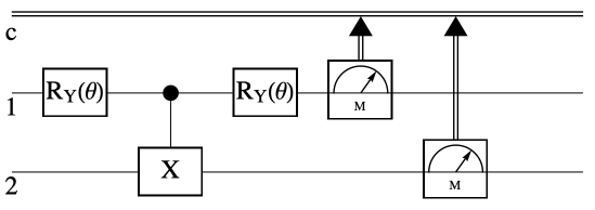
Probability results given the outcomes :
In[]:=
prob=FullSimplify[#,θ∈Reals]&/@qc[QuantumState[{"Register",2}]]["Probabilities"]
Out[]=

Return the efficiency rate
In[]:=
prob[|00〉]/(1-prob[|10〉])
Out[]=

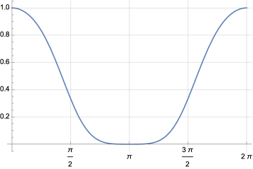
Plot the efficiency rate:
In[]:=
Plotprob[|00〉](1-prob[|10〉]),{θ,0,2π},
Out[]=
Increasing efficiency by using a series of beam splitters
Increasing efficiency by using a series of beam splitters
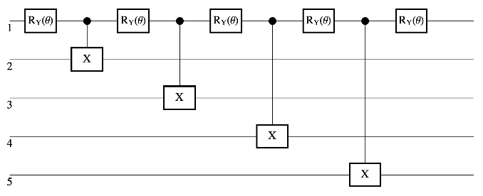
Define new quantum circuit using (θ):
R
y
In[]:=
qcN[θ_,m_Integer]:=With[{n=m-1},QuantumCircuitOperator[Flatten@{Table[{QuantumOperator[{"YRotation",θ}],QuantumOperator["CX",{1,i+1}]},{i,n}],QuantumOperator[{"YRotation",θ}]}]];
In[]:=
qcN[θ,5]["Diagram"]
Out[]=
Return the efficiency rate
η=(1-)
P
00,..,0
P
10,...,0
In[]:=
η[θ_,n_]:=Module[{ψr,ψt,ψf,pDet,pNul},(*|000,...,00〉*)ψr=QuantumState[{"Register",n}];(*|100,...,00〉*)ψt=QuantumOperator["X"]@QuantumState[{"Register",n}];(*finalstateattheendofthecicruit*)ψf=qcN[θ,n][ψr];(*innerproductswrtfinalstate*){pDet,pNul}=Abs[First@#["Dagger"][ψf]["StateVector"]]^2&/@{ψr,ψt};(*η*)pDet/(1-pNul)]
Plot the efficiency rate:
In[]:=
ListPlot[Table[EchoTiming@{n,N@η[π/n,n]},{n,2,12}],GridLines->All,AxesLabel{"#BS","η"},PlotLabel"η vs #Beam-Splitters, with θ=π/#BS"]
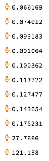
Out[]=
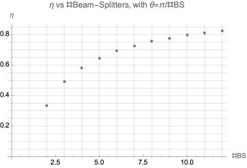
Note that the dimension of matrices is 2^#BS, so the calculations can get slow by increasing the number of qubits.
Hardy’s paradox
Hardy’s paradox
Paclet installation
Paclet installation
(*Note you need Mathematica version 12.3 or higher*)PacletUninstall/@PacletFind["Quantum*"];ClearAll["Wolfram`QuantumFramework`*","Wolfram`QuantumFramework`**`*"];PacletInstall[CloudObject@URLExpand@"https://wolfr.am/ZcOPnVar",ForceVersionInstall->True]<< Wolfram`QuantumFramework`
Out[]=