Introduction
Introduction
This project encompasses multiple undertakings. It includes geometric modelling of physical systems. It includes mathematical methods such as those found in the common reference book "Mathematical Methods for Physicists" by Arfken. It includes visual mathematics - using visual methods to perform complex calculations with minimal symbolic math and it includes quantum geometry. Certainly this project includes methods and concepts prevalent in NKS including space-time networks, nodes and connection algorithms.
It includes quantum reconstruction. This is an effort to rebuild quantum theory based on a few simple principles. This project extends Quantum Reconstruction into the macroscopic realm to include gravitation. From a few simple principles be able to build a prototypical model and detailed conception of our universe. At the same time the basic principles are well known and generally accepted. In the case of time being discrete, even quantized this is clearly indicated in our time keeping practices and a considerable amount of basic astronomical data supports this. This notion is put forth in NKS by Wolfram as well: "Just as for space, it is my strong belief that time is fundamentally discrete..." This is an effort to introduce these simple principes and develope a conceptul model of the universe.
It includes quantum reconstruction. This is an effort to rebuild quantum theory based on a few simple principles. This project extends Quantum Reconstruction into the macroscopic realm to include gravitation. From a few simple principles be able to build a prototypical model and detailed conception of our universe. At the same time the basic principles are well known and generally accepted. In the case of time being discrete, even quantized this is clearly indicated in our time keeping practices and a considerable amount of basic astronomical data supports this. This notion is put forth in NKS by Wolfram as well: "Just as for space, it is my strong belief that time is fundamentally discrete..." This is an effort to introduce these simple principes and develope a conceptul model of the universe.
Background
Background
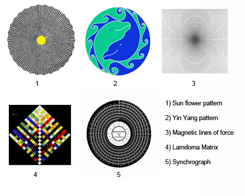
I have had the good fortune to be mentored by three pioneers in visual mathematics. Most notable is Mamikon who developed visual calculus to allow junior high through high schoolers to perform calculus using geometric methods with little or no symbolic mathematics. Bob Marshall taught me "synchrographics" resulting in the graphical computer shown below.This is a variation of the sieve of Eratosthenes showing patterns of highly composite numbers. Barbara Hero taught me about the Lamdoma matrix and harmonics. These all complimented my self directed studies which lead me to NKS, Synergetics and many other works in physics. Since high school visual mathematics was of great interest to me. This included geometry, the patterns of magnetic field lines, sunflowers and other patterns found in nature. My favorite artist has been MC Escher whose drawings are brimming with mathematics. A textbook illustration of a gravitational field with equi-spaced radial lines about a single pole was the starting point for this bi-radial matrix project. This was an early encounter of physics visualization. Here the number of equi-spaced radial lines corresponded to the mass and the gravitational field intensity I. Once the analogy of two masses required two sets of the equi-spaced radial lines in varying quantities intersecting to form interference patterns it became impractical to illustrate the numerous variations manually. Here my collaborator wrote a C++ program to allow the various parameters including the distance between the poles "A and"B". A section in the C++ code called "settable parameters" allowed me to make minor edits such as changing the number of equi-spaced rays from each pole, the distance between the poles to generate the numerous variations without re-writing C++ code. This was a huge help. It was a precursor to the "manipulate"functions I discovered later in Mathematica.
Mathematica Manipulate Interface
Mathematica Manipulate Interface
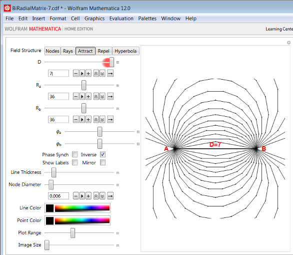
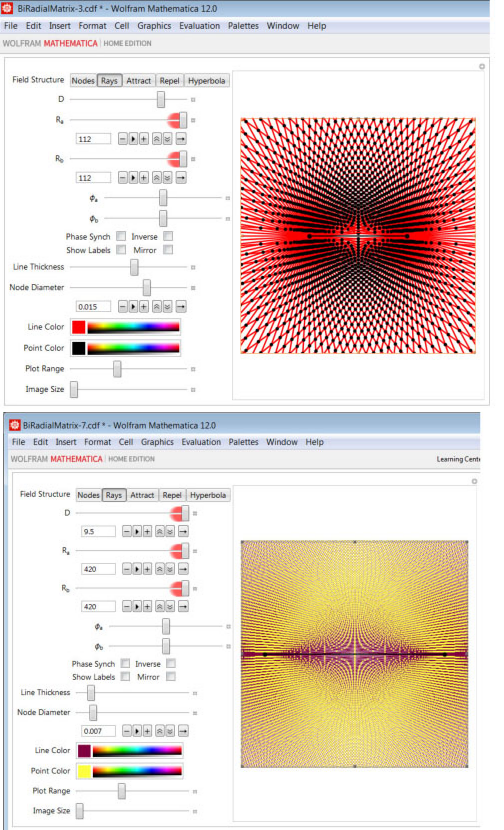
Here is the Mathematica manipulate interface for the bi-radial matrix. The parameters include the distance between the poles (D), the number of equi-spaced rays from each pole, Ra and Rb and the phase relation. There are other mathematical variables and graphical parameters such as the node diameter, line thickness, color and so on. These will be introduced in due course with the appropriate manipulate settings for diagrams.
Biradial Manipulate
Biradial Manipulate
Begin Package
Begin Package
BeginPackage["BiRadialMatrix`", {"GeneralUtilities`"}]
Needs[# <> "`", FileNameJoin[DirectoryName[$InputFileName], # <> ".wl" ]]& /@ { "BiradialPlot"}
Usage Statements
Usage Statements
SetUsage[BiradialManipulate, "BiradialManipulate[]"]
Begin Private
Begin Private
Begin["`Private`"] (* Begin Private Context *)
Manipulate
Manipulate
BiradialManipulate[] := DynamicModule[ pha = 0, phb = 0, phaseSync = False, phaseInverse = False, showLabels = False, mirrorRayNumbering = False , Manipulate[ BiradialPlot`makeBRMPlot[ d, ra, rb, pha, phb, rule, plotRange, "showPointLabels" -> showLabels, "lineThickness" -> thk, "nodeDiam" -> nodeDiam, "imgWth" -> width, "lineColor" -> lineColor, "pointColor" -> pointColor, "mirrorRayNumbering" -> mirrorRayNumbering ], {rule, "rays", "Field Structure"}, "nodes" -> "Nodes", "rays" -> " Rays ", "attract" -> " Attract ", "repel" -> " Repel ", "hyperbola" -> " Hyperbola " , {{d, 4, Style["D", 14]}, 1, 6, 1}, {{ra, 24, Style[Subscript["R", "a"], 14]}, 4, 60, 1}, {{rb, 24, Style[Subscript["R", "b"], 14]}, 4, 60, 1}, Item[Grid[ Style[Subscript["ϕ", "a"], 14], Dynamic[Manipulator[ Dynamic[pha, (pha = #; If[phaseSync, phb = ra / rb If[phaseInverse, -pha, pha]]) &], {N[-π / ra], N[π / ra]} ]] , Style[Subscript["ϕ", "b"], 14], Dynamic[Manipulator[ Dynamic[phb, (phb = #; If[phaseSync, pha = rb / ra If[phaseInverse, -phb, phb]]) &], {N[-π / rb], N[π / rb]} ]] ], Alignment -> Right], Item[Grid[ "Phase Synch", Checkbox[Dynamic[phaseSync]], "Inverse", Checkbox[Dynamic[phaseInverse]] , "Show Labels", Checkbox[Dynamic[showLabels]], "Mirror", Checkbox[Dynamic[mirrorRayNumbering]] ], Alignment -> Center], {{thk, 0.002, "Line Thickness"}, 0.001, 0.01, 0.001}, {{nodeDiam, 0.01, "Node Diameter"}, 0.005, 0.02, 0.001}, {{lineColor, Purple, "Line Color"}, ColorSlider}, {{pointColor, Black, "Point Color"}, ColorSlider}, {{plotRange, 6, "Plot Range"}, 2, 12, 1}, {{width, 400, "Image Size"}, 400, 800, 100} ], SaveDefinitions -> True(* , SynchronousInitialization -> False *) ]
Package footer
Package footer
End[] (* End Private Context *)EndPackage[]
Bi-Radial Matrix
Bi-Radial Matrix
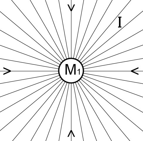
Diagram1
Diagram 1 depicts a gravitational field around a spherical mass M1 with uniform density. There can be as many or few lines as desired and they must be equi-spaced. As one researcher puts it: “The lines themselves are imaginary and do not actually exist; they are introduced as an aid to the understanding of gravitational forces and gravitational phenomenon.” For every location at the same distance from the center the field intensity i has the same magnitude. Later we will show how these equi-spaced radial lines relate to time and space and a geometric interpretation of “i” is derived. These radial lines-that don’t exist are really important and will be thoroughly investigated.
This model partially agrees with observation. As objects fall they converge towards a common center of gravity. The arrows indicate the equi-spaced radial lines all converge to a common center. The spacing of the lines shows the field is strongest at the surface. In this analogy the greater number of equi-spaced lines corresponds to a greater mass and stronger gravitational field. This analogy is only partial because the rate at which the rays diverge is a linear function where gravity is an inverse square function over distance. The surface area of a sphere or regular polyhedron varies per the square of the radius. This is a well known geometric model, Diagram 2 representing a gravitational field around a single mass.
This model partially agrees with observation. As objects fall they converge towards a common center of gravity. The arrows indicate the equi-spaced radial lines all converge to a common center. The spacing of the lines shows the field is strongest at the surface. In this analogy the greater number of equi-spaced lines corresponds to a greater mass and stronger gravitational field. This analogy is only partial because the rate at which the rays diverge is a linear function where gravity is an inverse square function over distance. The surface area of a sphere or regular polyhedron varies per the square of the radius. This is a well known geometric model, Diagram 2 representing a gravitational field around a single mass.
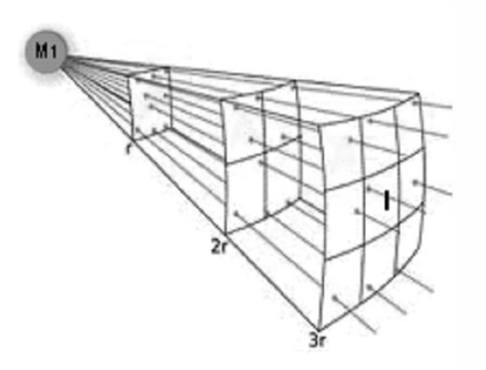
i=
1
2
r
Diagram 2
Is there a way to extend this analogy to describe an inverse square relation between TWO sizable masses and two interacting gravitational fields as described in Newton’s law of gravitation?
Is there a way to extend this analogy to describe an inverse square relation between TWO sizable masses and two interacting gravitational fields as described in Newton’s law of gravitation?
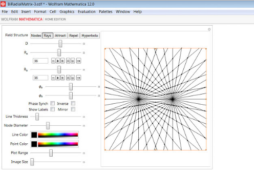
Diagram3-1
Description
Description
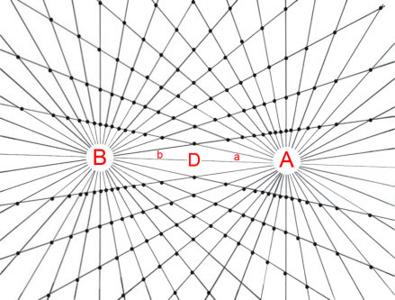
The Bi-radial Matrix consists of two sets of equi-spaced radial lines emanating from poles “A” and “B” separated by a distance “D” corresponding to two equal uniform density spherical masses. In this example the number of rays from each pole = 36 and the ray count can vary from very low to extremely high. Notice the nodes resulting from the intersections of the two sets of rays and the interior angles “a” and “b”. “a” represents ALL the included angles emanating from pole “A” and “b” represents all the included angles emanating from pole “B”. Notice the diamond shape in the interior and the trapezoids along with their changing shapes as they progress along the rays.
Basic Properties
Basic Properties
Diagram 3-2
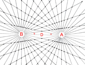
In diagram 3-2 the distance between poles A and B is decreased from diagram 3-1. From the principle of congruence it turns out that all the shapes and angles and relative proportions of the trapezoids remain the same. This applies on all scales. We can thus conclude that the bi-radial matrix is “invariant under spatial transformation”. This property will be important later. Notice in diagrams 3-1 and 3-2 the angles formed by the rays and notice the line segments along the rays. Both the line segments and the angles are “discrete” as in finite and distinct. The angles radiating from the poles A and B are “unitized” that is they are all the exact same unit of measure-“quantized” where as the line segments while they are discrete they are not quantized.
This is a crucial distinction. In the bi-radial matrix every angle within every trapezoid along with angles “a” and “b” are all quantized. All the side lengths of the trapezoids while they are discrete they are not quantized. There is a companion matrix with the exact inverse properties which I’m working on.
As the angles are quantized they can be mathematically described using counting numbers where the line segments being non-quantized require real numbers for their description. This fundamental relationship between the counting numbers and real numbers will be important later as it closely parallels the quantized vs non-quantized properties of the universe. There are other basic properties which are clarified with connection algorithms.
Connection Algorithms
Connection Algorithms
In diagram 4-1 the intersection nodes from diagram 3-1 are isolated. When I first encountered this array of nodes my first instinct was to determine the shortest path between pole “A” and pole “B” passing through the unoccupied nodes and to connect the nodes accordingly. This is the first connection algorithm relating to the bi-radial matrix. Diagram 4-1 begins this process. Diagram 4-2 and 4-3 continues. Completing this process until all the nodes are exhausted yields diagram 4-4. Diagram 4-1 Diagram 4-2 Diagram 4-3
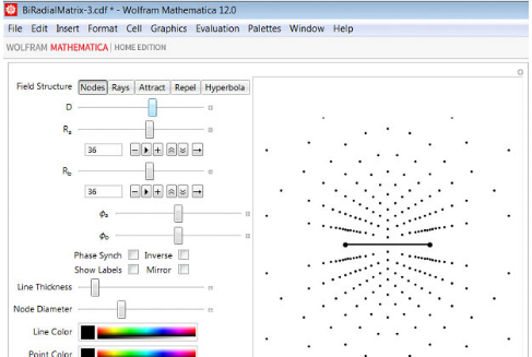
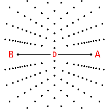
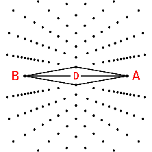
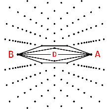
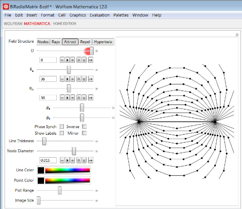
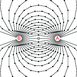
Diagram4-4Diagram4-5
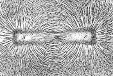
Diagram 4-5 shows actual iron filings under the influence of the attraction magnetic field from a permanent magnet. Diagram 4-6 shows diagram 4-4 highlighted in red superimposed over diagram 4-5 for direct comparison. We can casually observe the similarities and distinctions between the two patterns. Also it is known that the closer the field lines are to each other the stronger the force field in that vicinity. The further the spacing between the field lines the weaker the force field in that vicinity. This will be an important factor later. Recall as well that we are exploring a geometric analogy of gravitation and these “magnetic” lines of force emerged.
Diagram4-6
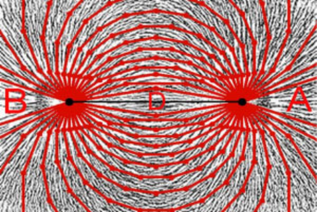
The similarities between the bi-radial matrix attraction lines and the tracings of actual magnetic attraction lines is highly significant and anything but a coincidence. More over it is striking to compare the results of the bi-radial matrix as shown in the previous diagrams with the description Wolfram gives in NKS regarding networks:
“A network system is fundamentally just a collection of nodes with various connections between these nodes and rules that specify how these connections should change from one step to the next....” Refer to diagrams 4-1 through 4-5 above. Further he states: “At any particular step in its evolution a network system can be thought of a little like an electric circuit, with the nodes of the network corresponding to the components of the circuit, and the connections to the wires joining these components together....”
The are several connection algorithms which relate to the underlying network of nodes based on the bi-radial matrix. It can be casually observed in the special case of the bi-radial matrix when the number of rays from pole “A” and pole “B” are equal that there is a set of nodes which falls along a vertical “V” axis, perpendicular to and bisecting the “D” segment. Here the next connection algorithm is as follows: Starting from pole “A” and pole “B” what are the paths which come into the closest proximity to the “V” axis passing through the unoccupied
nodes?
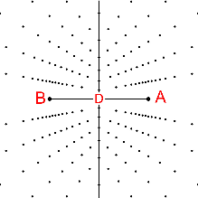
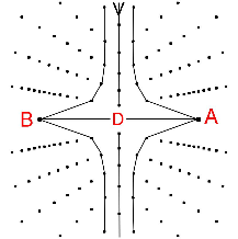
Diagram5-1Diagram5-2Diagram5-3
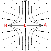
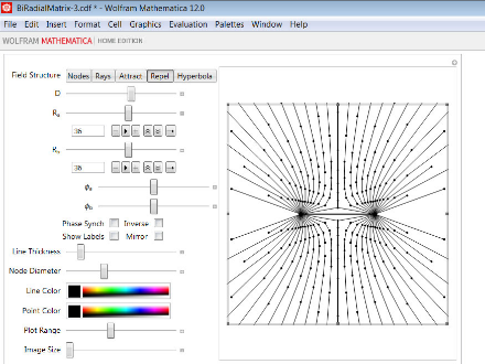
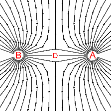
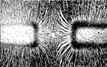
Diagram5-4Diagram5-6
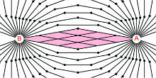
Diagrams 5-1 through 5-3 show this process taken to two iterations. Diagram 5-4 shows the results after all the nodes are occupied and diagram 5-5 shows iron filings under the influence of a magnetic repulsion field between two like poles of separate permanent magnets. Diagram 5-6 shows diagram 5-4 highlighted in red superimposed over diagram 5-5 for direct comparison. Here again we regard the similarities in the two respective patterns as highly significant. The results of our research suggest that the bi-radial structure relates directly to space and time and that the bi-radial matrix is a fundamental space-time network.
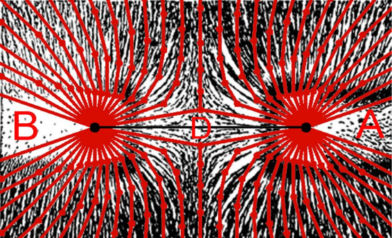
Figure 5-7
Diagrams 4-6 and 5-6 reveal similarities between magnetic attraction and repulsion “lines of force” and geometric field lines derived from the bi-radial matrix. These prototypical field structures were derived by applying specific connection algorithms to the bi-radial matrix. Are there mathematical relationships which can be derived from the geometry? Can we describe the field lines mathematically and are there inverse square relationships which extends the scope of this geometric analogy?
Deriving Inverse Square Relations From First Principles
Deriving Inverse Square Relations From First Principles
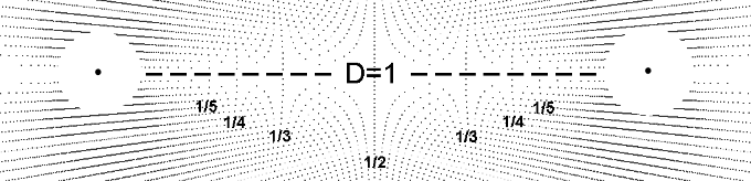
The original geometric analogy dealt with gravitation. The derivation of the attraction and repulsion lines suggests a relationship with electromagnetism. Each of these forces obey an inverse square law based on distance. Is there an inverse square relationship over distance within the geometry of the bi-radial matrix? Diagram 6-1 shows the poles separated by unit distance and in this diagram the shaded diamond is designated as unit area. When the distance is doubled in diagram 6-2 the area "A" of the interior diamond increases by a factor of four (4).
When the distance between the poles is tripled from diagram 6-1 the area of the interior diamond shape increases by a factor of nine (9). It is known that the closer the spacing of the field lines in a magnetic field the stronger the force is in that region and the further the spacing between the field lines the weaker the force is in that region. Hence the larger the central diamond shape the further the spacing between the field lines in that region. Thus an inverse square relation over distance is present in the bi-radial matrix extending the geometric analogy with respect to force. This describes force in terms of a quantized interference pattern.
When the distance between the poles is tripled from diagram 6-1 the area of the interior diamond shape increases by a factor of nine (9). It is known that the closer the spacing of the field lines in a magnetic field the stronger the force is in that region and the further the spacing between the field lines the weaker the force is in that region. Hence the larger the central diamond shape the further the spacing between the field lines in that region. Thus an inverse square relation over distance is present in the bi-radial matrix extending the geometric analogy with respect to force. This describes force in terms of a quantized interference pattern.
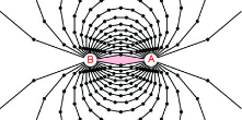
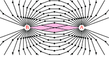
Diagram6-1Diagram6-2Diagram6-3
Alternative expression of inverse square relation over distance.
Alternative expression of inverse square relation over distance.
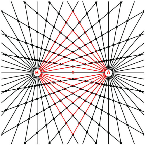
Diagram7-1
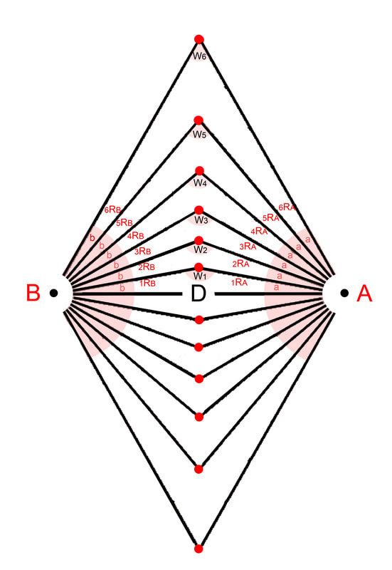
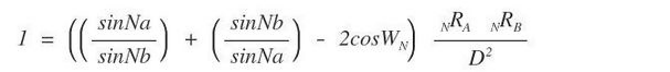
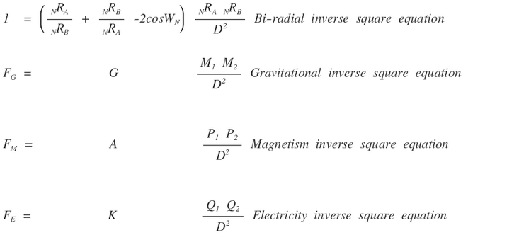
Diagram 2 is the basis of the inverse square law which applies to a wide range of phenomenon from gravity emanating from a single source, radiation, sound and any single point source which spreads its influence equally in all directions. Diagrams 6-1, 6-2 and 6-3 reveal inverse square relation over distance corresponding to two interacting fields and relating to the central diamond region. Diagrams 7-1 highlights the interior radial segments where the number of rays from each pole A=36 and B=36. This model is the geometric analogy to represent phenomenon emanating from two origins such as two large scale gravitational masses with two centers of mass, magnetism with two poles. Like diagram 1 can the bi-radial symmetry describe a general inverse square equation over distance D? Diagram 7-2 Diagram 7-2 labels the interior angles and radial segments as highlighted in diagram 7-1 with variables for reference in the following equation. Mathematical variables A = number of equi-spaced rays from pole A B = number of equi-spaced rays from pole B a = associated angles around pole A b = associated angles around pole B D = distance between pole A and pole B WN = Central angle NRN = Radial segments I = field intensity* From the law of cosines equation 3-1 describes the triangles in diagrams 11 highlighted in red and isolated in diagram 12. Equation1-1 Below equation 3-1 is compared to the known inverse square force equations relating to gravity, magnetism and electricity: We can note the similarities and differences between equation 3-1 and the fundamental inverse square force equations. Our research indicates the similarity between these equations is not a coincidence. That this is a consequence of the space time structure in the vicinity of these forces being bi-radial. Note the field intensity I requires further clarification later. In the next article space and time are defined with respect to the components of the bi-radial matrix showing how it represents a space-time network. Further properties including a scaling mechanism and harmonic structure are covered.
Visual Arts
Visual Arts
“Visual Arts” are among the groups I am addressing. There are many ways the manipulate interface can create stunning graphical images. Thus far we have dealt mostly with the mathematical parameters. There are several graphical parameters such as line thickness, color of lines and nodes available to create stunning graphics revealing harmonic patterns which can be appreciated visually and intuitively.
Summary
Summary
A network was derived from two sets of equi-spaced rays forming an interference pattern called the bi-radial matrix to visualize the gravitational interaction between two ideal equal uniform density spherical masses. The features of this matrix can be varied with the manipulate function in Mathematica to illustrate a variety of physical phenomenon. This is a logical extension of a previously established geometric visualization and analogy to gravitation. This matrix is invariant under spatial transformation and has other important properties relating to three fundamental forces. This interference pattern revealed a set of intersection nodes within the network. Two connection algorithms were implemented deriving prototypical models of attraction and repulsion field structures from first principles. Both geometric and mathematical expressions of the inverse square relations were derived from the bi-radial matrix. The manipulate interface has additional functions for graphic illustration for the visually oriented. Further research covers several other permutations of the matrix, a bi-radial coordinate system to further the analysis and relating this to current trends in physics.
Biradial Plot Functions
Biradial Plot Functions
Begin Package
Begin Package
BeginPackage["BiradialPlot`", {"GeneralUtilities`"}]
Needs[# <> "`", FileNameJoin[DirectoryName[$InputFileName], # <> ".wl" ]]& /@ "VectorGeometry"
Usage Statements
Usage Statements
SetUsage[makeBRMPlot, "makeBRMPlot[d$, ra$, rb$, pa$, pb$, rule$, plotRange$]"]
Begin Private
Begin Private
Begin["`Private`"] (* Begin Private Context *)
makeBRMPlot
makeBRMPlot
(* Combined function to generate final plot from set of input parameters *)Options[finalizePointLabels] = {"mirrorRayNumbering" -> False}Options[makeBRMPlot] = Join[ Options[finalizePointLabels], "showPointLabels" -> False, "lineThickness" -> 0.001, "nodeDiam" -> 0.01, "imgWth" -> Automatic, "lineColor" -> Purple, "pointColor" -> Black ]
makeBRMPlot[ d_, ra_, rb_, pa_, pb_, rule_, plotRange_, opts:OptionsPattern[]] := Module[ showPointLabels, lineThickness, nodeDiam, imgWth, lineColor, pointColor, pole1, pole2, leftlines, rightlines, leftlines2, rightlines2, posIntPnts, negIntPnts, intPnts, negIntPntsAdj, posAttractPnts, negAttractPnts, attractPnts , (* Retrieve Options *) showPointLabels, lineThickness, nodeDiam, imgWth, lineColor, pointColor = OptionValue["showPointLabels"], OptionValue["lineThickness"], OptionValue["nodeDiam"], OptionValue["imgWth"], OptionValue["lineColor"], OptionValue["pointColor"] ; (* Pole positions *) pole1 = {-d / 2, 0}; pole2 = {d / 2, 0}; (* Generate rays *) leftlines = generateRadialLinesLeft[pole1, ra, pa]; rightlines = generateRadialLinesRight[pole2, rb, pb]; (* Split rays point upward from rays pointing downward *) leftlines2 = GroupBy[leftlines, #[[2, 2]] > 0&]; rightlines2 = GroupBy[rightlines, #[[2, 2]] > 0&]; (* Ray intersection points *) posIntPnts = intersectRaySets[leftlines2[True], rightlines2[True]]; negIntPnts = intersectRaySets[leftlines2[False], rightlines2[False] ]; intPnts = Join[posIntPnts, negIntPnts]; negIntPntsAdj = KeyMap[ rb - #[[1]] + If[pb == 0, 0, 1], ra - #[[2]] + If[pa == 0, 0, 1] &, negIntPnts]; (* Apply the Rule *) If[rule != "rays", posAttractPnts = makePoints[posIntPnts, rule]; negAttractPnts = makePoints[If[rule != "hyperbola", negIntPnts, negIntPntsAdj ], rule]; attractPnts = addPoles[posAttractPnts, negAttractPnts, pole1, pole2 , rule]; ]; (* Display the plot *) Show[ Which[ rule == "nodes", makeNodePlot[intPnts, d, plotRange, nodeDiam, imgWth, pointColor ] , rule == "rays", makeBiradialPlot[leftlines, rightlines, intPnts, d, plotRange, lineThickness , nodeDiam, imgWth, lineColor, pointColor] , True, linesPlot[intPnts, attractPnts, d, plotRange, lineThickness, nodeDiam , imgWth, lineColor, pointColor] ], If[showPointLabels, makeIntersectionLabels[ finalizePointLabels[ intPnts, ra, rb, FilterRules[{opts}, Options[finalizePointLabels]] ] ] , {} ] ] ];
Inner Functions
Inner Functions
(* Check if a point is on a ray *)pointOnRayQ[p2_, {p1_, v1_}] := VectorGeometry`scalarProject[p2 - p1, v1] > 0;
(* Compute the intersection of two rays *)intersectRaysJJM[{r1_, r2_}] := Module[{ln1, ln2, ip}, ln1 = List @@ r1; ln2 = List @@ r2; ip = VectorGeometry`intersectLinesTwo[ln1, ln2]; If[SameQ[ip, {}], Return[{}] ]; If[pointOnRayQ[ip, ln1] && pointOnRayQ[ip, ln2], ip , {} ] ]
(* Generate the radial lines of the left pole *)generateRadialLinesLeft[cent_, num_, phase_] := Module[{dt, angles}, (* define radial incremement *) dt = N[2 π / num]; (* Sort lines taking into account the phase offset *) angles = Sort[Replace[ Mod[Table[n dt + phase, {n, Range[num]}], 2 π], x_ /; x < 10.^-15 -> Nothing, 1 ]]; (* Generate the radial lines as HalfLines (lines which start at a point and continue on indefinitely) *) Association[ # -> HalfLine[cent, {Cos[angles[[#]]], Sin[angles[[#]]]}] & /@ Range[Length[angles]]] ]
(* Generate the radial lines of the right pole *)generateRadialLinesRight[cent_, num_, phase_] := Module[{dt, angles}, dt = N[2 π / num]; angles = Sort[Replace[ Mod[Table[n dt + phase, {n, Range[num]}], 2 π], x_ /; x < 10.^-15 -> Nothing, 1 ]]; Association[ # -> HalfLine[cent, {Cos[π - angles[[#]]], Sin[π - angles[[#]]]}] & /@ Range[Length[angles]]] ]
(* Find the intersections of two ray sets *)intersectRaySets[leftlines_, rightlines_] := Module[{pairs}, pairs = Outer[ ({First[#1], First[#2]} -> {Last[#1], Last[#2]})&, Normal[rightlines], Normal[leftlines] ]; pairs = Flatten[pairs]; Association[Replace[ ParallelMap[First[#] -> intersectRaysJJM[Last[#]]&, pairs], ({a_, b_} -> {}) -> Nothing, 1 ]] ]
primaryLabelStyle[text_] := Style[text, Bold, Red, 18];
(* Graphically label the pole locations and insert the D line *)poleLocations[d_] := Graphics[ Black, PointSize[0.02], Point /@ {{-d / 2, 0}, {d / 2, 0}}, Thick, Line[{{-d / 2, 0}, {d / 2, 0}}], Text[primaryLabelStyle["D=" <> ToString[d]], {0, 0.05 d}], Text[primaryLabelStyle["A"], {-0.6 d, 0}], Text[primaryLabelStyle["B"], {0.6 d, 0}] ];
(* Label the ray intersection points *)makeIntersectionLabels[intpnts_] := Graphics[{Blue, KeyValueMap[Text[Most[#1], #2, {0, -1.2}]&, intpnts]}];
(* Label the rays starting from the positive D line and rotating upward *)makeRayLabels[leftlines_, rightlines_] := Graphics[ KeyValueMap[ Text[#1, First[#2] + 2 * Last[#2], {-1.5, 1.5}]&, leftlines ], KeyValueMap[ Text[#1, First[#2] + 2 * Last[#2], {-1.5, 1.5}]&, rightlines ] ];
(* Produce a plot of the intersection nodes *)makeNodePlot[intPnts_, d_, plotRange_, nodeDiam_:0.01, imgWth_:Automatic , pointColor_:Black] := Show[Graphics[pointColor, PointSize[nodeDiam], Point /@ Values[intPnts ], PlotRange -> plotRange, ImageSize -> imgWth], poleLocations[d]];
(* Produce plot of the rays and their intersections *)ClearAll[makeBiradialPlot];makeBiradialPlot[leftlines_, rightlines_, intPnts_, d_, plotRange_, lineThickness_ :0.001, nodeDiam_:0.01, imgWth_:Automatic, lineColor_:Purple, pointColor_ :Black] := Show[Graphics[ lineColor, Thickness[lineThickness], Values[leftlines], Values[rightlines], pointColor, PointSize[nodeDiam], Point /@ Values [intPnts] , PlotRange -> plotRange, ImageSize -> imgWth], poleLocations[d]];
(* Procude fully labelled plot of the rays and their intersections *)makeLabeledBiradialPlot[leftlines_, rightlines_, d_, plotRange_] := Module[{intpnts}, intpnts = intersectRaySets[leftlines, rightlines]; Show[ makeBiradialPlot[leftlines, rightlines, intpnts, d, plotRange], makeRayLabels[leftlines, rightlines], makeIntersectionLabels[intpnts], PlotRange -> plotRange, ImageSize -> Large ] ]
(* Get the points that make up the lines of different field structures. The primary function used here is GroupBy *)makePoints[inpnts_, rule_String] := GroupBy[KeyValueMap[Switch[rule, "attract", Plus , "repel", Subtract , "hyperbola", Divide ] @@ #1, #1, #2&, inpnts], First];
(* Connect the lines to the poles. For much of this it is easiest to divide the plane into 4 quadrants (positive-negative | left-right) *)addPoles[posPnts_, negPnts_, pole1_, pole2_, rule_String] := Switch[rule, "attract", (* Add poles at the start and end of each complete line - if the line goes outside of range do not link back to a pole *) Join[ <|ToString[#] <> "P" -> Join[If[First[posPnts[#][[1, 2]]] == 1, {{#, {0, 0}, pole1}} , {} ], posPnts[#], If[Last[posPnts[#][[-1, 2]]] == 1, {{#, {0, 0}, pole2}} , {} ]]& /@ Keys[posPnts]|>, <|ToString[#] <> "N" -> Join[If[Last[negPnts[#][[1, 2]]] == Max[Values [negPnts[[All, 1, 2, 2]]]], {{#, {0, 0}, pole2}} , {} ], negPnts[#], If[First[negPnts[#][[-1, 2]]] == Max[Values[negPnts [[All, 1, 2, 1]]]], {{#, {0, 0}, pole1}} , {} ]]& /@ Keys[negPnts]|> ] , "repel", (* At poles to the start of each line *) Join[ <|ToString[#] <> "PL" -> Join[{{#, {0, 0}, pole1}}, posPnts[#]]& /@ Select[Keys[posPnts], # <= 0&]|>, <|ToString[#] <> "PR" -> Join[{{#, {0, 0}, pole2}}, posPnts[#]]& /@ Select[Keys[posPnts], # >= 0&]|>, <|ToString[#] <> "NL" -> Join[negPnts[#], {{#, {0, 0}, pole1}}]& /@ Select[Keys[negPnts], # >= 0&]|>, <|ToString[#] <> "NR" -> Join[negPnts[#], {{#, {0, 0}, pole2}}]& /@ Select[Keys[negPnts], # <= 0&]|> ] , "hyperbola", (* Do not add poles *) Join[ <|ToString[#] <> "P" -> posPnts[#]& /@ Keys[posPnts]|>, <|ToString[#] <> "N" -> negPnts[#]& /@ Keys[negPnts]|> ] ];
(* Plot the field lines with tunable parameters *)linesPlot[intPnts_, linePoints_, d_, plotRange_, lineThickness_:0.001 , nodeDiam_:0.01, imgWth_:Automatic, lineColor_:Purple, pointColor_:Black ] := Show[Graphics[lineColor, Thickness[lineThickness], Line[#[[All, 3]] ]& /@ Values[linePoints], pointColor, PointSize[nodeDiam], Point /@ Values[intPnts] ], poleLocations[d], PlotRange -> plotRange, ImageSize -> imgWth];
finalizePointLabels[intPnts_Association, ra_Integer, rb_Integer, opts:OptionsPattern[]] := <|KeyValueMap[ If[#2[[2]] > 0, Append[#1, "Upward"], Append[If[OptionValue["mirrorRayNumbering"], {rb, ra} - #1, #1], "Downward"] ] -> #2 &, intPnts ]|>
Package footer
Package footer
End[] (* End Private Context *)EndPackage[]
Vector Geometric Functions
Vector Geometric Functions
Begin Package
Begin Package
BeginPackage["VectorGeometry`", {"GeneralUtilities`"}]
Usage Statements
Usage Statements
SetUsage[scalarProject, "scalarProject[u$, v$] gives the length of the scalar projection of u$ onto v$."]SetUsage[intersectLinesTwo, "intersectLinesTwo[{p$, v$}, {q$, u$}] intersects the parametric line p$ + k$ v$ with the line q$ + h$ u$ using similar triangles"]
Begin Private
Begin Private
Begin["`Private`"] (* Begin Private Context *)
Vector Geometric Functions
Vector Geometric Functions
(* ||u||^2 *)norm2[u_List] := u . u
(* area of a triangle use Heron's formula *)triangleArea[a_, b_, c_] := Sqrt[(b + c - a) (a + b - c) (a + c - b) (a + b + c)] / 4
(* give the length of the scalar projection of u onto v *)scalarProject[u_List, v_List] := u . v / Norm[v]
(* give the component of vector u in the direction of vector v *)vectorProject[u_List, v_List] := (u . v) / (v . v) v
(* decompose u into two vectors, the first parallel to v, the second perpendicular to v *)orthogonalDecompose[u_List, v_List] := With[{w = vectorProject[u, v]}, {w, u - w} ]
(* project the point q onto the line p + k v *)projectPointLine[q_List, {p_List, v_List}] := p + vectorProject[q - p, v];
(* determine the distance between the point q and the line p + k v*)distPointLine[q_List, {p_List, v_List}] := Norm[q - projectPointLine[q, {p, v}]];
(* determine the cosine of the angle between the two vectors u, v*)cosineBetween[u_List, v_List] := (u . v) / (Norm[u] Norm[v])
angleBetween[u_List, v_List] := ArcCos[cosineBetween[u, v]]
(* intersect the parametric line p + k v with the line q + h u using similar triangles *)intersectLinesTwo[{p_List, v_List}, {q_List, u_List}] := Module{d, c, h, l}, d = distPointLine[p, {q, u}]; c = distPointLine[p + d v, {q, u}]; If[Abs[d - c] < 10^-9, Return[{}] ]; (* Use similar triangles *) Ifd > c, h = d + c d (d - c); Return[p + h v]; , h = d^2 (c - d); Return[p - h v]; ;
Package footer
Package footer
End[] (* End Private Context *)EndPackage[]