Just saw this quite interesting post on twitter. I would like to show one way to create this plot with several built-in functions and one WFR function:

ResourceFunction[“AccumulateApply”] is very handy in this case:
In[]:=
Out[]=
{f[1],f[1,2],f[1,2,3],f[1,2,3,4]}
It takes the incremental length of arguments and this is what we need: the approximation of π using incremental depth of layers of continued fraction:
In[]:=
cfPoints={Denominator[#],RealAbs[#-π]}&/@[FromContinuedFraction[{##}]&,ContinuedFraction[π,12]];
The best numerator associated with a given denominator is solved by this set inequalities
q
p
1)
2)
π-3-q/p>0
2)
π-3-(q+1)/p<0
Then the minimum error is found by computing the differences again by either or , choosing the min absolute value of the two:
q
q+1
approx=With[{r=Range[2*^6]},{r,Min[Abs[Floor[#*(π-3)]/#-π+3.],Abs[(Floor[#*(π-3)]+1)/#-π+3.]]&/@r}//Transpose];
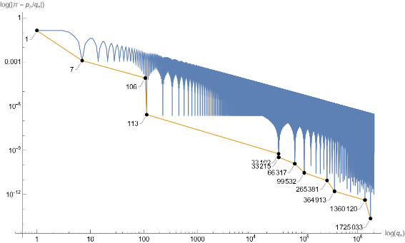
Put the data into the plot function and generate the log-log plot of denominator of nearest rational number vs. error of estimation. The lower bound is connected by continued fraction approximation. The label using the same convention in the twitter.
In[]:=
ListLogLogPlot[{approx,Callout[#,#[[1]],Left,LeaderSize{20,240Degree,5}]&/@cfPoints},Joined->True,Epilog{PointSize[0.01],Point/@Log[cfPoints]},AxesLabel{"",""},LabelStyle14,PerformanceGoal"Speed"]
log()
q
n
log(||)
π-/
p
n
q
n
Out[]=