Machine Learning in chemistry education: carbonyl multiclass classification
by Elizabeth Thrall
Version Date: October 28, 2021
by Elizabeth Thrall
Version Date: October 28, 2021
Abstract
Abstract
This notebook implements a machine learning classification algorithm for functional group identification in vibrational spectroscopy. In chemistry, functional groups are particular arrangements of atoms and bonds that appear in many different molecules. This analysis focuses on the carbonyl functional group, which contains a carbon atom double bonded to an oxygen atom. The carbonyl functional group itself appears in a number of other functional groups, including ketones and carboxylic acids.
Functional groups have distinct signatures in vibrational spectroscopy due to their characteristic arrangement of atoms and bonds. The problem of functional group identification entails predicting which functional groups are present in a particular molecule given its spectrum. This notebook walks through the steps to train a multiclass machine learning classification model to predict whether molecules contain ketones, carboxylic acids, or other carbonyl groups based on their infrared (IR) absorption spectra. The model performance is then evaluated using a test data set.
This activity was developed at Fordham University for a physical chemistry laboratory course taken by junior and senior chemistry majors.
Objectives
Objectives
◼
Gain proficiency in reading and modifying Mathematica code in the notebook environment.
◼
Build machine learning multiclass classification models to predict whether a molecule contains a ketone, a carboxylic acid, or another type of carbonyl functional group using IR spectroscopy data.
Initialization
Initialization
The Synthetic Minority Oversampling Technique (SMOTE) function is provided as an initialization cell and will be loaded when you first evaluate anything in this notebook. It will be used during the data preprocessing step.
Define SMOTE function
Define SMOTE function
Get Data
Get Data
We will need a training dataset and a test dataset. These data are computational IR absorption spectra obtained from the Alexandria Library (https://www.nature.com/articles/sdata201862).
◼
In this case, all molecules in both datasets contain a carbonyl group, so the three classes are: ketone, carboxylic acid, or other carbonyl group.
◼
The training data is saved in three separate files: one with a label indicating whether or not a ketone is present, one with a label indicating whether or not a carboxylic acid is present, and one with a label indicating whether or not another carbonyl is present (i.e., whether neither ketone nor carboxylic acid are present).
◼
The test data set is stored in a single file with three columns corresponding to the labels for ketone, carboxylic acid, and other.
◼
In all cases, the presence of a particular group is indicated by the label 1 and the absence by the label 0.
Run the following code cell to retrieve the training and test data for this exercise:
In[]:=
{ketone,cbxlAcid,other,testData}=Import["https://raw.githubusercontent.com/elizabeththrall/MLforPChem/main/MLforvibspectroscopy/Data/"<>#,"Dataset",HeaderLines1]&/@{"multi_ketone.csv","multi_cbxl_acid.csv","multi_other.csv","multi_test.csv"};
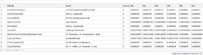
Let’s display the contents of a few of these variables to familiarize ourselves with their structure. First, the first 10 rows of the ketone training data:
In[]:=
ketone[[1;;10]]
Out[]=
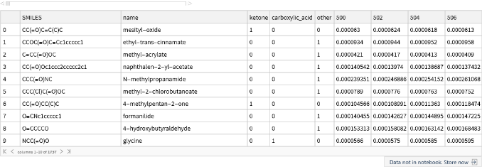
Then the test data:
In[]:=
testData[[1;;10]]
Out[]=
Data Preprocessing
Data Preprocessing
We will need to preprocess the data before carrying out the machine learning analysis. We will perform four preprocessing steps:
◼
Split the attribute and label
◼
Normalization
◼
Thresholding
◼
Data balancing
Split Attribute and Label
Split Attribute and Label
Notice that the training and test data contain the molecule name and label in addition to the spectral data. Our first task is to separate the information about whether or not the molecule contains a carbonyl (the attribute we want to predict, let’s call it “Y”) from the spectral intensities (the input features that we will use to make a decision, let’s call it “X”). We will also convert this into a form that is more amenable to machine learning analysis, where our goal is to find a function that describes Y = f(X).
We begin by defining a function that splits the attributes and labels:
We begin by defining a function that splits the attributes and labels:
◼
The first argument in the square brackets following the function name represents the data to be split.
◼
The second argument, startX, represents the column index where the frequency data starts. If you don't provide this argument, the function uses a default value of 5.
◼
The third argument, endX, represents the column index where the frequency data end. If you don’t provide this argument, the function uses a default value of -1 (the last element)
◼
The fourth argument, startY, represents the first column containing the label data. If you don’t provide this argument, the function uses a default value of 4.
◼
The fifth argument, endY, represents the last column containing the label data. If you don’t provide this argument, the function uses a default value of 4.
◼
As an example, if the frequency data in train starts in column 5 and the label data is in column 4, you would write: splitXY[train, 5, -1 , 4].
In[]:=
splitXY[data_Dataset,startX_:5,endX_:-1,startY_:4,endY_:4]:=With[{x=data[[All,startX;;endX]]//Values//Normal,y=data[[All,startY;;endY]]//Values//Normal//If[startYendY,(First/@#),#]&},MapThread[(#1#2)&,{x,y}]]
This function returns a list of entries, where each item is of the form x (list of inputs) y (output value). This is one of the many formats that Mathematica can use for machine learning tasks.
Plotting Spectra
Plotting Spectra
Before continuing, let’s look at the spectra of a few molecules to see what they look like. We will use the splitXY function but i general we will not look at the lists of data that it returns directly, and so it is useful to suppress the output by putting a semicolon at the end of the line. You can choose which spectra to plot by changing the index values contained in the exampleIndices list below:
In[]:=
exampleIndices={1,7};(*entry1doesnothaveaketone,entry7does*)examples=splitXY[ketone[[exampleIndices]]];(*extractourtrainingdata*)names=ketone[[exampleIndices,"name"]]//Normal;(*extractthecorrespondingnames*)
In[]:=
ListLinePlot[examples,DataRange->{500,4000},PlotRangeAll,PlotLegends{"not ketone","ketone"}]
Out[]=
We can add legend and other information by setting the various options of the ListLinePlot (see the documentation for examples and explanations):
In[]:=
ListLinePlot[examples,(*thedata*)PlotLegendsPlaced[names,{Right,Top}],(*othersettings...*)PlotRangeAll,DataRange{500,4000},FrameLabel{"Frequency ()","Intensity"},PlotTheme"Scientific"](*arrowsareusedtopassoptionvaluestoListLinePlot*)
-1
cm
Out[]=
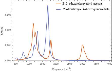
Let’s wrap this up into a function to facilitate reuse:
llp[data_,names_:None]:=ListLinePlot[data,PlotLegendsPlaced[names,{Right,Top}],PlotRangeAll,DataRange{500,4000},FrameLabel{"Frequency ()","Intensity"},PlotTheme"Scientific"]
-1
cm
Normalization
Normalization
In practice, different IR spectra may be recorded at different molecular concentrations, so the absolute intensities may not be directly comparable. Therefore we will normalize the data before carrying out the analysis.
We will apply a type of normalization called min-max normalization to each "instance" (i.e., molecule) and update the data.
◼
For each molecule, the spectral intensities will be scaled to range from 0 to 1.
◼
We will define a function called normalize to carry out this normalization process. Specifically, we will define the function, normalize to act on each entry in list. Then we will define this function as “Listable” meaning that it will apply to each entry in a list.
In[]:=
normalize[x_y_]:=Rescale[x]ySetAttributes[normalize,Listable]
Apply Threshold
Apply Threshold
We expect that intensities near 0 won’t provide much useful information for the classification. Therefore we will choose a threshold intensity and set all intensity values below the threshold equal to 0.
We will define a function called applyThreshold to apply the threshold chosen above to the training and test data; conveniently we can make use of the built-in Threshold function; the only trick is to apply it only to our “inputs” and keep our “outputs” the same:
In[]:=
applyThreshold[thresholdVal_:0.22][x_y_]:=Threshold[x,{"Hard",thresholdVal}]yapplyThreshold[thresholdVal_:0.22][data_List]:=applyThreshold[thresholdVal]/@data
Putting it together
Putting it together
Now we can apply the three preprocessing functions to the training and test data.
In[]:=
{trainKetone,trainCbxl,trainOther}=(applyThreshold[0.2]@normalize@splitXY[#])&/@{ketone,cbxlAcid,other};test=applyThreshold[0.2]@normalize@splitXY[testData,7,-1,4,6];
Data Balancing
Data Balancing
The three classes (ketone, carboxylic acid, and other carbonyl group) are imbalanced in the training dataset. Thus we need to balance the data before training a machine learning model. We will use the synthetic minority oversampling technique (SMOTE) for this data balancing step. Because there are three sets of training data, we will need to use SMOTE on each one separately.
In[]:=
{balancedKetone,balancedCbxl,balancedOther}=SMOTE/@{trainKetone,trainCbxl,trainOther};
Building Random Forest Machine Learning Models
Building Random Forest Machine Learning Models
We will use the Random Forest machine learning algorithm for this multiclass classification task. The first step is model training using the training data. Instead of training a single model, we will train three different models: one for the ketone training data, one for the carboxylic acid training data, and one for the other carbonyl training data. We will train three additional models using the corresponding balanced training data. We will store the trained models in an Association:
In[]:=
(*constructanassociationoftrainingsetnamesandexamples*)trainingSets=AssociationThread[{"ketone","cbxl","other","ketone (balanced)","cbxl (balanced)","other (balanced)"},{trainKetone,trainCbxl,trainOther,balancedKetone,balancedCbxl,balancedOther}];(*maptrainingprocessovereachtrainingset;turnoffprogressreportingpanel*)models=Classify[#,Method"RandomForest",TrainingProgressReportingNone]&/@trainingSets;
Note that each model is now accessible by its key:
In[]:=
models["ketone"]
Out[]=
ClassifierFunction
This allows us to look up a model from the association, and apply it to new data to generate predictions:
In[]:=
examples=trainKetone[[1;;2,1]];(*twoexampleentries,retainingonlytheinputs*)models["ketone"][examples](*applythemodeltoeachoftheexamples,generatingaresult*)
Out[]=
{0,0}
Testing Machine Learning Models
Testing Machine Learning Models
Now we will use the trained machine learning models for label prediction on the test dataset. We will use each of the six trained models on the same test input data. We will store the predicted labels in the Association predictions, with the keys describing each of the models
In[]:=
(*generatepredictonsforeachmodelintheinstructorset*)predictions=#[test[[All,1]]]&/@models;(*exampleoutput...justtotakealook*)predictions["ketone (balanced)"]
Out[]=
{1,0,0,0,0,0,1,0,0,0,0,0,1,0,0,0,0,0,0,0,0,0,0,0,1,0,0,0,0,0,0,0,1,0,0}
We can also obtain the probability of a given label (i.e., how confident the model is in the prediction). Let’s take a look at a quick example. Suppose that we wanted to apply our classifier to a few examples from our ketone training set, trainKetone. As we saw previously we can apply the classifier function, stored in the models Association, with the key “ketone”, and use it to generate the predicted label:
In[]:=
examples=trainKetone[[1;;2,1]];models["ketone"][examples]
Out[]=
{0,0}
We can also provide the classifier function with an optional second argument, which will report the probabilities for each type of class, in the form of an Association:
In[]:=
models["ketone"][examples,"Probabilities"]
Out[]=
{00.92748,10.0725198,00.917275,10.0827249}
Alternatively, if we are just interested in the probability that it is “1” (is a ketone”) then we can use the “Probability”outcome label form to only report those outcomes:
In[]:=
models["ketone"][examples,"Probability"1]
Out[]=
{0.0725198,0.0827249}
Having seen how the pieces work, let’s evaluate the probabilities for each of the individual models, storing the results in an association, probabilities, whose keys describe which model is used to make the prediction:
In[]:=
probabilities=#[test[[All,1]],"Probability"1]&/@models;
After completing this calculation, we can examine the results:
In[]:=
(*demo:whatarethemodels?*)Keys[probabilities](*example:whataretheprobabilitiesassignedbytheketonemodel?*)probabilities["ketone"]
Out[]=
{ketone,cbxl,other,ketone (balanced),cbxl (balanced),other (balanced)}
Out[]=
{0.105373,0.0630492,0.0630492,0.0827249,0.0725198,0.0630492,0.225829,0.0827249,0.0936737,0.0936737,0.0827249,0.0725198,0.105373,0.282439,0.0725198,0.105373,0.0827249,0.131038,0.0725198,0.0936737,0.0827249,0.0630492,0.365545,0.105373,0.117827,0.0630492,0.387374,0.0827249,0.117827,0.0827249,0.477218,0.0630492,0.431913,0.191353,0.590483}
Multiclass Classification
Multiclass Classification
Now that we have the probabilities of each label prediction, we can determine the most probable label as the one with the highest probability. For example, if the probabilities are:
◼
Ketone: 0.20
◼
Carboxylic acid: 0.79
◼
Other carbonyl: 0.15
...then the final prediction would be carboxylic acid. (Note that the probabilities do not have to sum to 1 here, as they are probabilities for each independent yes-no prediction.)
Run the code block below to determine the most probable prediction and display a Dataset comparing the probabilities, the prediction, and the actual label (i.e., the “truth”); each of the categories is assigned an integer code 1=ketone, 2 = carboxylic acid, 3=other:
In[]:=
results=With[(*extractnamesandtruelabelsfromoriginaldataimport*){names=Normal@Values@testData[[All,2;;3]],(*moleculenameandSMILESinformation*)trueLabels=Normal@Values@testData[[All,4;;6]],(*getthetruevalues*)p=Transpose@Lookup[probabilities,{"ketone (balanced)","cbxl (balanced)","other (balanced)"}]},(*extractprobabilitiesasatriple*)With[(*findtheplacewhereeachislargesttogenerateaclasslabel*){predict=ResourceFunction["PositionLargest"]/@p,(*highestprobabilitypredictionlabel*)truth=ResourceFunction["PositionLargest"]/@trueLabels},(*predicttrueoutcomelabel*)ResourceFunction["DatasetWithHeaders"][(*mergetheresultsandreturnaDataset*)MapThread[Join,{names,p,Transpose[{predict}],Transpose[{truth}]}],{"SMILES","name","ketone","carboxylic_acid","other","predict","truth"}]]]
Out[]=
Although there is only one way for a prediction to be correct, there are multiple ways for a prediction to be incorrect here because there are multiple labels. Run the code block below to generate a table showing the different combinations of correct and incorrect predictions; the first column indicates the predicted label, the second column shows the true label, and the final column is the number of occurrences:
In[]:=
tabulatedResults=KeySort@results[GroupBy["predict"],CountsBy["truth"]];Dataset[tabulatedResults,MaxItems->{3,3}]
Out[]=
To make this more readable, we can replace the outcome keys (1, 2, 3) with the corresponding labels (“ketone”, “cbxl”, “other”):
In[]:=
Dataset[ResourceFunction["KeyReplace"][Normal[tabulatedResults],{1->"ketone",2->"cbxl",3->"other"},All],MaxItems->{3,3}]
Out[]=
This data can be arranged in the format of a confusion matrix like the ones from the first lab, where the rows are the predictions and the columns are the true values. (But to create more confusion, sometimes these matrices are presented with the rows and columns swapped.):
In[]:=
confusionMatrix[data_]:=With[{labels=Keys@Normal@KeySort@data[Counts,"truth"]},Table[Length@data[Select[(#truth==trueLabel)&&(#predict==predictLabel)&]],{predictLabel,labels},{trueLabel,labels}]]confusionMatrix[results]//MatrixForm(*applytoourdata*)
Out[]//MatrixForm=
2 | 1 | 1 |
0 | 5 | 3 |
3 | 1 | 19 |
Visualizing inaccuracies
Visualizing inaccuracies
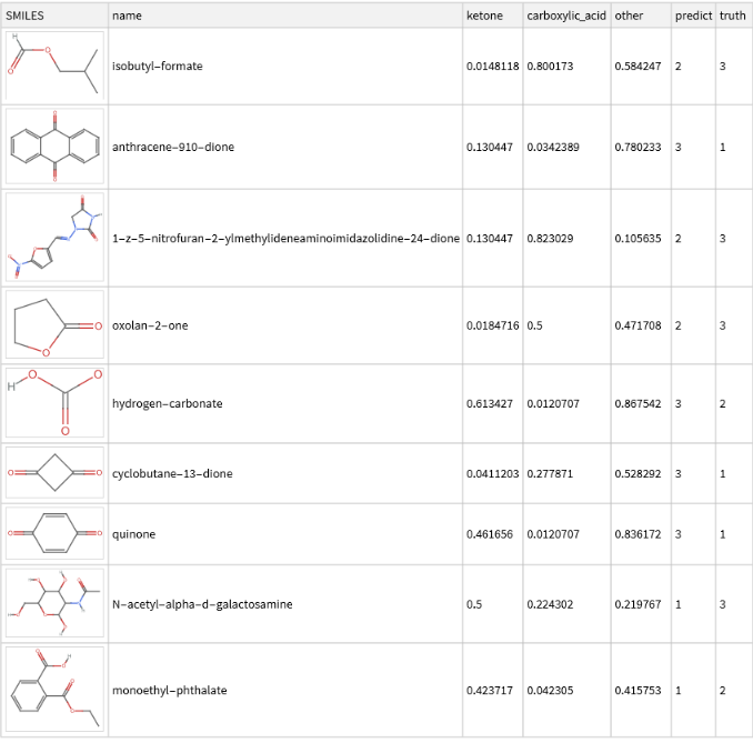
It can also be helpful to visualize where the predictions differ from the true values. Run the below code to visualize the result:
In[]:=
molPlot[smiles_String]:=MoleculePlot@Molecule[smiles];results[Select[#["truth"]≠#["predict"]&],{"SMILES"molPlot}](*applytocurrentlistofresults*)
Out[]=
Assessing Overall Model Performance
Assessing Overall Model Performance
To determine the overall performance of the model, we can calculate an overall accuracy score, equal to the total number of correct predictions divided by the total number of predictions. Run the code blocks below to determine and display the overall accuracy:
In[]:=
(*defineafunction*)computeAccuracy[results_]:=With[{nTotalItems=Length[results],(*howmanytestitems?*)nCorrectItems=Length@Select[results,#["truth"]#["predict"]&]},(*howmanyagree?*)SetPrecision[nCorrectItems/nTotalItems,4]](*computefractionandroundto4decimalplaces*)(*applytoourresults*)computeAccuracy[results]
Out[]=
0.7429
Alternatively, the dataset functionality can be used to compute this in a more direct way:
In[]:=
computeAccuracy[results_Dataset]:=With[{averageCorrect=results[Mean,Boole[#truth==#predict]&]},(*reducetobooleanvariablesandcomputemean*)SetPrecision[averageCorrect,4]](*computeaverageandroundto4decimalplaces*)(*applytoourresults*)computeAccuracy[results]
Out[]=
0.7429
We can also determine accuracy scores for each of the three classes. For example, the ketone class accuracy score would be the total number of correct ketone predictions divided by the total number of true ketones in the test data. We do this by grouping the results by the truth labels and then computing the accuracy on each subset. Run the code blocks below to determine and display the accuracy for each (true) class:
In[]:=
tabulatedAccuracy=computeAccuracy/@results[GroupBy["truth"]]//KeySort;Dataset[ResourceFunction["KeyReplace"][Normal[tabulatedAccuracy],{1->"ketone",2->"cbxl",3->"other"},All],MaxItems->{3,3}]
Out[]=
Next Steps
Next Steps
The analysis in this notebook can be modified or extended in a number of different ways:
◼
Changing data preprocessing or machine learning analysis parameters
◼
Using another machine learning classification algorithms (such as k-Nearest Neighbors or Naive Bayes) instead of Random Forest
◼
Extending the analysis to other carbonyl-containing functional groups (such as esters or aldehydes)
◼
Using the same multiclass classification framework to distinguish between the IR spectra of carbonyls and other functional groups (such as alcohols, amines, alkenes, etc)
◼
Using the trained machine learning model for functional group prediction in experimental or computational IR spectra datasets
Acknowledgments
Acknowledgments
We thank Mark Hendricks and Kedan He for testing this activity and providing helpful feedback. We also thank the physical chemistry laboratory students at Fordham University and Whitman College for their participation.