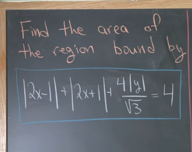
This blog is again inspired by the interesting lecture from Dr Michael Penn's YouTube Channel (one of the best math channel and approaching 150K subs quickly!) . My goal here is to show a little more generalized result using interactive built-in WL functions. Typically, it is going to show the limit of p-norm as p approaches infinity with a geometric application.
Analysis
Analysis
Because we have three absolute value adding together, it is nature to link to space and using Norm function to generalize this sum. Without the second argument, Norm function returns regular Euclidean metrics.
p
L
Norm[{a,b,c}]
Out[]=
2
Abs[a]
2
Abs[b]
2
Abs[c]
If the second argument is 1, we have something presented in the problem
Norm[{a,b,c},1]
Out[]=
Abs[a]+Abs[b]+Abs[c]
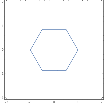
To visualize the region in Michael’s lecture, the following one-liner just works
ContourPlotNorm2x-1,2x+1,*y,1==4,{x,-2,2},{y,-2,2}
4
3
Out[]=
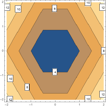
which is an item of the list of hexagon contours. The numbered text boxes are the value on the contour for .
C
C|2x-1|+|2x+1|+||
4y
3
ContourPlotNorm2x-1,2x+1,*y,1,{x,-2,2},{y,-2,2},ContourLabelsFunction[{x,y,z},Text[Framed[z],{x,y},BackgroundWhite]]//Rasterize
4
3
Out[]=
To make the area computation easily sweep through various values, I defined the following function. Note that I convert any P value greater than a given threshold to infinity, beyond which I don’t see much difference in visualization and numeric result once the variable passes.
P
In[]:=
normFunc[p_]:=Norm2x-1,2x+1,*y,If[p<=11,p,Infinity];
4
3
This is where p is at infinity
normFunc["Infinity"]=normFunc[100]
Out[]=
MaxAbs[-1+2x],Abs[1+2x],
4Abs[y]
3
I can compute symbolic result are by Integrate and Boole function. Boole makes the “height” 1 on region bounded by the inequality and 0 elsewhere. There is another value gives symbolic result quickly,which represents the area of ellipse .Cache the special values
p2
{initArea,ellipticArea,finalArea}=Integrate[Boole[normFunc[#]<=4],{x,-2,2},{y,-2,2}]&/@{1,2,"Infinity"}
Out[]=
,π,6
3
3
2
7
4
3
2
3
Define the area function for p-sweeping later
In[]:=
Clear[areaFunc]
areaFunc[p_?NumericQ]:=Whichp==1,initRes,p==2,ellipticArea,1<p<=11,NIntegrateBooleNorm2x-1,2x+1,*y,p<=4,{x,-2,2},{y,-2,2},,p>11,infRes
4
3
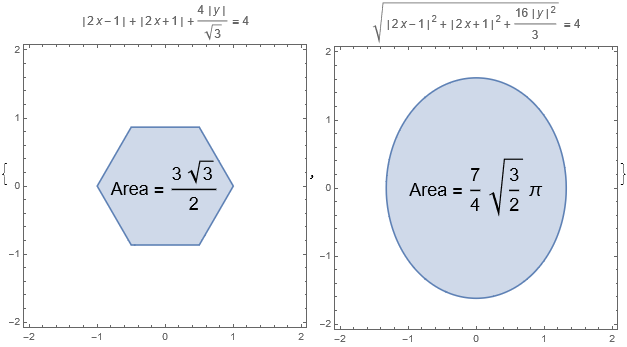
I can show the area of the given problem using the results above with RegionPlot, which highlights the bounded region
Rasterize[With[{p=#},RegionPlot[normFunc[p]<=4,{x,-2,2},{y,-2,2},PlotPoints25,PlotLabelRow[{normFunc[p]," = ",4}],Epilog{Inset[Style[Row[{"Area = ",areaFunc[p]}],18],{0,0}]},ImageSize300]]&/@{1,2}]
Out[]=
Before I create the animation, I set some points to see how the bounded area changes with
In[]:=
xValue=Range[10]~Join~{100};
Compute the bounded area at 1-norm, 2-norm, and so on.
In[]:=
areas=areaFunc/@xValue;
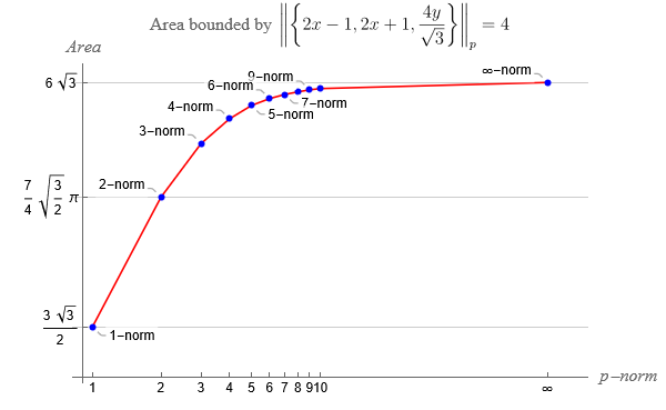
Use ListLogLinearPlot to change the x axis to logarithm scale to handle a mixture of large and small numbers. Callout is helpful to read coordinates with the absent of vertical grid lines.
ListLogLinearPlotCallout[#,Style[Row[{#[[1]],"-norm"}/.{100->Infinity}],12]]&/@Transpose[{xValue,areas}],PlotLabelStyleRow"Area bounded by ",
,FontFamily"Times New Roman",16,Ticks{Transpose[{xValue,xValue/.{100∞}}],{initArea,ellipticArea,finalArea}},TicksStyleDirective[12],AxesLabel(Style[#1,FontFamily"Times New Roman",16,Italic]&)/@{"p-norm","Area"},GridLines{None,{initArea,ellipticArea,finalArea}},PlotStyleRed,JoinedTrue,AxesOrigin{0,1},MeshAll,MeshStyleBlue,ImageSize600,ImagePadding{{65,70},{25,10}}//Rasterize

Out[]=
Let’s check if the limit is correct or not. Use the definition of the p-norm and solve the equation algebraically
normFunc["Infinity"]
Out[]=
MaxAbs[-1+2x],Abs[1+2x],
4Abs[y]
3
Reduce[normFunc["Infinity"]<=4,{x,y},Reals]
Out[]=
-≤x≤&&-
3
2
3
2
3
≤y≤3
The boundaries, simply two vertical segments and two horizontal segments, form a rectangle with side lengths equal 3 and . Thus the area is
3*2*
3
Out[]=
6
3
This result is identical to my previous symbolic integration.
Create Animation
Create Animation
As you can see from the beginning of the blog, every frame of the animation is the combination of two plots. They are threaded with Column function to align perfectly in the vertical direction.
◼
Top: Sweeping across many values of with RegionPlot
p
frames1=Table[RegionPlot[normFunc[p]<=4,{x,-2,2},{y,-2,2},PlotPoints25,PlotLabelRow[{normFunc[p]," = ",4}],Epilog{Inset[Style[Row[{"Area = ",areaFunc[p]}],18],{0,0}]},ImagePadding{{Automatic,Automatic},{Automatic,20}}],{p,1,15,1/5}];
◼
Top: Sweeping across many values of with ContourPlot. You want to specify the Contours options so when plot function changes, the color across different plots means the same value
p
frames2=Table[ContourPlot[normFunc[p],{x,-2,2},{y,-2,2},Contours->Range[4,8,1/2],ExclusionsNone],{p,1,15,1/5}];
Combine the plots and create a new frame
frames3=MapThread[Column[{#1,#2},BaseStyle->ImageSizeMultipliers->1]&,{frames1,frames}];
Export frames to a GIF file or ready to use ListAnimate inside notebook.
Export["pnorm.gif",frames3]
Summary
Summary
◼
Norm function handles -norm easily
p
◼
The given inequality envelopes larger area with larger value, and it comes with a limit
p
◼
ContourPlot plots a curve or path or a family of such objects with satisfying a certain implicit quantitative relationship
{x,y}
◼
RegionPlot works similar to the contour version, but usually requires inequality to fill up a bounded region
◼
Integrate and Boole function works together to integrate over a region satisfying given inequality
◼
NIntegrate with advanced options saves large amount of time of computing over sophisticated region with complex integrands