Problem
Problem
In[]:=
<<MaTeX`
Out[]=

The following URL links to the background of the problem, originally posted by Suzuki Kantaro on his Youtube Channel
In[]:=
SystemOpen["https://youtu.be/tKq3I4IakvA"]
I will present the visual solution (one shot death blow) to the problem first and then explain the observation with some algebra. ComplexPlot was introduced to Mathematica in V12.0 and is updated in V12.1 with a very useful syntax sugar. It is a very powerful tool to understand the topology of holomorphic and meromorphic function over complex plane.
One Line Solution
One Line Solution
Just take a look at the equation itself, we can conclude that the norm of the cannot be too large. Otherwise the norm of would grow much faster than the linear multiplication of the norm of , which can also be verified with basic calculus. We may roughly guess that a rectangular region with side less than 2 and centered at origin encloses all possible solutions for =8>22-1.
z
3
z
z
3
2
In[]:=
GraphicsRow[cp=ComplexPlot[z^3-2*Abs[z]+1,{z,2},ColorFunction#,PlotLegendsAutomatic]&/@{Automatic,"GlobalAbs"}]
Out[]=
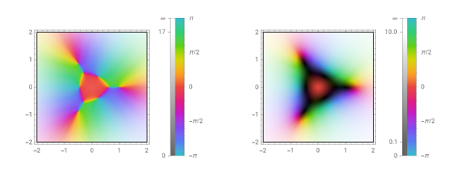
The plot on the right hand side in our graphics row is the same as the left one with additional shading. The darker a region is covered, the smaller the norm of the complex number in that particular region.
If you take a look at the plot on the left, there are some tiny dark dots on the plane with which rainbow of colors surrounds. Let’s do a quick count and we shall have 9 such points, as shown below
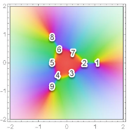
Notice that points 1, 2 and 5 lie on horizontal line with or on real number line, we have to drop them according to the domain specified in the equation. Thus the number of valid solutions is simply
Im[z]=0
In[]:=
9-3//Framed
Out[]=
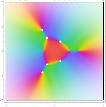
To obtain the precise location, symbolically Reduce the equation and overlay the dots onto our previous diagram with ComplexListPlot. These roots perfectly matches our observation in the last plot.
In[]:=
Show[cp[[1]],ComplexListPlot[z/.Transpose@{((List@@Reduce[z^3-2Abs[z]+10&&Abs[Im[z]]>0,z])/.EqualRule)},PlotStyle{White,PointSize[0.02]},PlotRange2]]
Out[]=
How to Read ComplexPlot and Domain Coloring
How to Read ComplexPlot and Domain Coloring
There are many functions you can insert into ComplexPlot. But for function with finite number of zeros or poles, you only need to understand the following five plots and basic modulo arithmetic. Then you can easily generalize the following examples to higher order cases.
In[]:=
GraphicsRow@{ComplexPlot[z,{z,2}],ComplexPlot[-z,{z,2}],ComplexPlot[z^2,{z,2}],ComplexPlot[1/z,{z,2}],ComplexPlot[1/z^2,{z,2}]}
Out[]=
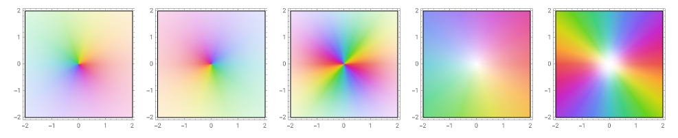
Plots are numbered 1 to 5, from left to right
In[]:=
SetOptions[Plot,AxesLabel{"Arg(z)","Arg(f(z))"},ExclusionsStyleDirective[Blue,Dashed],PlotLegends{"arg(z) ↦ arg(z)","arg(z) ↦ arg(f(z))"}];
1
.Reference Plot: hue convention and principal argument are initially defined. Say you pick a point {1,1}, the corresponding complex number is , therefore we define orange as π/4 in this convention.
1+
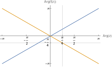
2
.Angular Shift: in the plot if we pick the same point {1,1} for complex number , the color is very close to blue. Referring to plot 1, the corresponding region is in third quadrant around . This result is convincing because know the output rotates any complex 180 degree anticlockwise. Notice the coloring in plot 2 is also a rotation of 180 degree, which is just a angular shift.
1+
-3π/4
z↦-z
In[]:=
Plot[{θ,Mod[θ+π,2π,-π]},{θ,-π,π},Ticks->{{-π,-π/2,0,π/4,π/2,π},{-π,-3π/4,π}},GridLines{{π/4},{-3π/4}}]
Out[]=
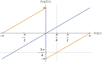
The direction of color sweeping sequence is the same as plot 1
3
.Repeating zero/ winding number = 2: the principal argument mapping is just the following simple modular algorithm
In[]:=
Plot[{θ,Mod[2*θ,2π,-π]},{θ,-π,π},Ticks->{{-π,-π/2,0,π/4,π/2,π},{-π,π/2,π}},GridLines{{π/4},{π/2}}]
Out[]=
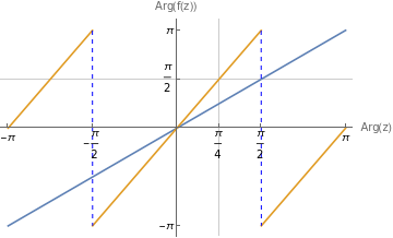
For example we use the same complex number with . The color at that spot is green. Referring to plot 1, green is close to pointing upward which is 90 degree. This result matches the plot right above. We notice the direction of color sweeping sequence is the same as plot 1 and each color occurs exactly twice. We can easily extend the argument to power of three:
1+
arg(z)=π/4
In[]:=
Plot[{θ,Mod[3*θ,2π,-π]},{θ,-π,π},Ticks->{{-π,-π/2,0,π/2,π},{-π,π}}]
Out[]=
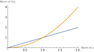
The other observation is that the dark region is larger than that in plot 1. When , <r and curve is sort of “flat”. For region outside of unit circle, the norm grows rapidly, so does the brightness.
r=z<1
2
r
In[]:=
Plot[{r,r^2},{r,0,2},PlotStyleThick,PlotLegends"Expressions",AxesLabel{"Norm of z","Norm of f(z)"}]
Out[]=
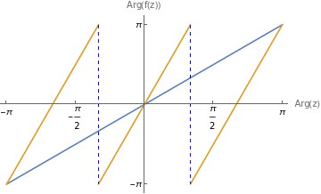
4
.Non repeating pole: we have . Therefore its principal argument is the negative version
1/z=/(z·)=/
z
z
z
2
r
In[]:=
Plot[{θ,Mod[-θ,2π,-π]},{θ,-π,π},Ticks->{{-π,-π/2,0,π/4,π/2,π},{-π,-π/4,π}},GridLines{{π/4},{-π/4}}]
Out[]=
Also the slope is negative, which means the direction of color wheel is reversed, winding number = . Also the brightness is opposite to plot 1, as the center is brighter than edge. This is simply because the norm of 1/z is hyperbolic.
-1
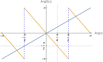
5
.Repeating pole: we have . Use the same argument in 3 and 4, and sample value , we have
1/==
2
z
2
()
z
2
(z·)
z
2
()
z
4
r
1+
In[]:=
Plot[{θ,Mod[-2θ,2π,-π]},{θ,-π,π},Ticks->{{-π,-π/2,0,π/4,π/2,π},{-π,-π/2,π}},GridLines{{π/4},{-π/2}}]
Out[]=
Remark
Remark
◼
Use ComplexPlot to identify zeros and poles for target function
◼
Link winding number to plots of modulo algorithm
◼
◼