Installation
Installation
The simplest way to automatically download and install the latest release of IGraph/M is to evaluate the following line in Mathematica:
In[]:=
Get["https://raw.githubusercontent.com/szhorvat/IGraphM/master/IGInstaller.m"]
The currently installed versions of IGraph/M are: {}
Installing IGraph/M is complete: PacletObject.
It can now be loaded using the command
To install IGraph/M manually, or to install a different version than the latest one, download the.paclet file from the GitHub releases page, and install it using the PacletInstall Mathematica function. For example, ifIGraphM-0.6.2.paclet was downloaded into the directory ~/Downloads, then evaluate
Needs["PacletManager`"]PacletInstall["~/Downloads/IGraphM-0.6.2.paclet"]
If the .paclet file was downloaded to a different location, adjust the path above accordingly.
It is not necessary to uninstall old versions before installing a new one.
A more detailed guide for installing packages distributed in the paclet format is available on StackExchange.
Once installed, test that it works with a few simple commands:
It is not necessary to uninstall old versions before installing a new one.
A more detailed guide for installing packages distributed in the paclet format is available on StackExchange.
Once installed, test that it works with a few simple commands:
In[]:=
<<IGraphM`
Out[]=
IGraph/M 0.6.2 (July 25, 2022) |
Evaluate |
In[]:=
IGVersion[]
Out[]=
IGraph/M 0.6.2 (July 25, 2022)igraph 0.9.9-68-g0c33f892b (Jul 25 2022)Microsoft Windows (64-bit)
In[]:=
Graph[GraphData["DodecahedralGraph"],EdgeStyle->Directive[Thick,Opacity[1]],VertexStyle->Black]//IGEdgeMap[ColorData[109],EdgeStyle->IGEdgeColoring]
Out[]=
Showcase
Showcase
Featured examples
Featured examples
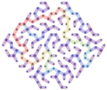
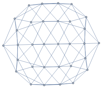
Create a random maze as a random spanning tree of a regular lattice confined to a hexagon, and colour it according to betweenness centrality:
In[]:=
g=IGMeshGraph@IGLatticeMesh["CairoPentagonal",Polygon@CirclePoints[6,6]];t=IGRandomSpanningTree[g,VertexCoordinates->GraphEmbedding[g],GraphStyle->"ThickEdge"];IGEdgeMap[ColorData["Rainbow"],EdgeStyle->IGEdgeBetweenness/*Rescale,t]
Out[]=
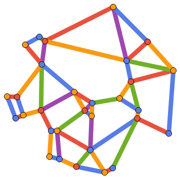
Compute and visualize a minimum vertex and edge colouring of the Gabriel graph of a set of spatial points:
In[]:=
IGGabrielGraph[RandomPoint[Disk[],30],GraphStyle->"Monochrome",VertexSize->1,EdgeStyle->Thickness[1/40]]//IGVertexMap[ColorData[106],VertexStyle->IGMinimumVertexColoring]//IGEdgeMap[ColorData[106],EdgeStyle->IGMinimumEdgeColoring]
Out[]=
Mesh/graph conversions
Mesh/graph conversions
Let us take a polyhedral mesh.
In[]:=
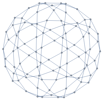
mesh=PolyhedronData["TruncatedIcosahedron","BoundaryMeshRegion"]
Out[]=

It is easy to convert it to a graph.
In[]:=
g=IGMeshGraph[mesh]
Out[]=

We could also easily convert it to a face-adjacency graph, or an edge-adjacency graph
In[]:=
(*facetofaceadjacency,preservingcoordinates*)IGMeshCellAdjacencyGraph[mesh,2,VertexCoordinatesAutomatic]
Out[]=

In[]:=
(*edgetoedgeadjacency*)IGMeshCellAdjacencyGraph[mesh,1]
Out[]=
Graph symmetries
Graph symmetries
This is a very symmetric graph. The graph structure looks exactly the same when viewed from any vertex. In other words, the graph is vertex-transitive.
In[]:=
IGVertexTransitiveQ[g]
Out[]=
True
The same is not true for edges though.
In[]:=
IGEdgeTransitiveQ[g]
Out[]=
False
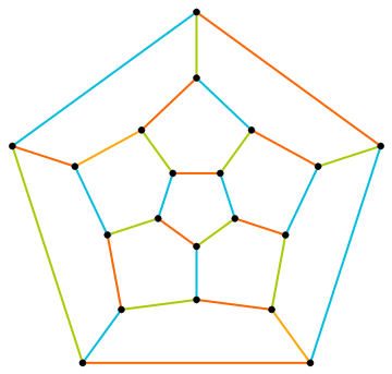
There are in fact two types of edges: those separating a hexagonal face from a pentagonal one, and those separating two hexagonal faces. We can visualize them:
In[]:=
HighlightGraph[g,GroupOrbits[IGBlissAutomorphismGroup[g],EdgeList[g]]]
Out[]=

How many symmetries (automorphisms) does the graph have?
In[]:=
IGBlissAutomorphismCount[g]
Out[]=
120
Planarity
Planarity
This is also a planar graph.
In[]:=
IGPlanarQ[g]
Out[]=
True
We can find all its faces.
In[]:=
IGFaces[g]
Out[]=
{{1,41,47,31,6,10},{1,10,15,27,59},{1,59,9,23,19,41},{2,42,20,24,11,60},{2,60,28,16,12},{2,12,8,32,48,42},{3,57,5,13,25,43},{3,43,49,15,10,6},{3,6,31,21,57},{4,44,26,14,7,58},{4,58,22,32,8},{4,8,12,16,50,44},{5,57,21,33,29,56},{5,56,7,14,13},{7,56,29,34,22,58},{9,53,11,24,23},{9,59,27,51,30,53},{11,53,30,52,28,60},{13,14,26,36,35,25},{15,49,37,39,51,27},{16,28,52,40,38,50},{17,18,55,46,45,54},{17,54,47,41,19},{17,19,23,24,20,18},{18,20,42,48,55},{21,31,47,54,45,33},{22,34,46,55,48,32},{25,35,37,49,43},{26,44,50,38,36},{29,33,45,46,34},{30,51,39,40,52},{35,36,38,40,39,37}}
Each list in the result contains the ordered vertices of a face.
We can also compute a Tutte layout of the graph, with an arbitrary choice of outer face. A planar graph can be drawn with any of its faces being the outer face.
In[]:=
IGLayoutTutte[g,"OuterFace"->{4,58,22,32,8}]
Out[]=
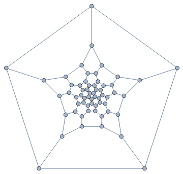
In a typical Tutte layout, the vertices are often closely packed in the middle. It would be nice to space them out. supports edge weights. We can simply compute an initial layout, then assign the Euclidean distance of each edge’s endpoints as its weight, finally compute a weighted Tutte layout.
IGLayoutTutte
In[]:=
IGLayoutTutte@IGDistanceWeighted@IGLayoutTutte[g]
Out[]=
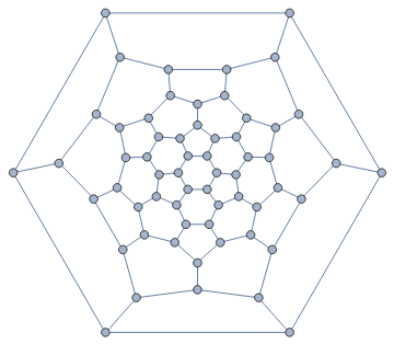
We can even transform the edge weights to adjust between a closely spaced and a loosely spaced layout. This is easy with .
IGEdgeMap
In[]:=
Manipulate[IGLayoutTutte@IGEdgeMap[#^alpha&,EdgeWeight]@IGDistanceWeighted@IGLayoutTutte[g],{{alpha,1},0.5,2}]
Out[]=
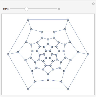
While Mathematica has built in, selecting the desired outer face or using weights is only possible with IGraph/M.
GraphLayout"TutteEmbedding"
We can not only find the faces of this planar graph, we can also compute its dual graph.
In[]:=
dualG=IGDualGraph[g]
Out[]=
Or find a combinatorial embedding, i.e. a counterclockwise ordering of neighbours around each vertex.
In[]:=
IGPlanarEmbedding[g]
Out[]=
1{41,10,59},2{42,60,12},3{57,43,6},4{44,58,8},5{13,57,56},6{3,10,31},7{58,14,56},8{4,32,12},9{53,23,59},10{6,15,1},11{53,60,24},12{8,2,16},13{5,14,25},14{13,7,26},15{10,49,27},16{12,28,50},17{18,54,19},18{17,20,55},19{17,41,23},20{18,24,42},21{57,31,33},22{32,58,34},23{19,9,24},24{23,11,20},25{13,35,43},26{14,44,36},27{15,51,59},28{16,60,52},29{33,34,56},30{52,53,51},31{21,6,47},32{22,48,8},33{29,21,45},34{29,46,22},35{25,36,37},36{35,26,38},37{35,39,49},38{36,50,40},39{37,40,51},40{39,38,52},41{19,47,1},42{20,2,48},43{25,49,3},44{26,4,50},45{33,54,46},46{45,55,34},47{41,54,31},48{42,32,55},49{43,37,15},50{44,16,38},51{39,30,27},52{40,28,30},53{30,11,9},54{47,17,45},55{48,46,18},56{29,7,5},57{21,5,3},58{22,4,7},59{27,9,1},60{28,2,11}
Graph colouring
Graph colouring
Let us compute a minimum vertex colouring of the dual graph. Since it is planar, we know that it is possible in at most 4 colours.
In[]:=
Graph3D[dualG,VertexSizeLarge]//IGVertexMap[ColorData[100],VertexStyleIGMinimumVertexColoring]
Out[]=

It was indeed necessary to use 4 colours.
In[]:=
IGChromaticNumber[dualG]
Out[]=
4
The original graph, however, can be both vertex-coloured and edge-colored using only 3 colours.
In[]:=
{IGChromaticNumber[g],IGChromaticIndex[g]}
Out[]=
{3,3}
The vertex colouring of the dual graph of a polyhedral skeleton is actually a face colouring of the polyhedron. Let us visualize the colouring like this.
In[]:=
SetProperty[{mesh,{2,All}},MeshCellStyleColorData[100]/@IGMinimumVertexColoring@IGMeshCellAdjacencyGraph[mesh,2]]
Out[]=

Proximity graphs
Proximity graphs
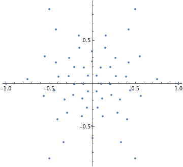
Earlier, we computed a nice layout for this graph. Can we reconstruct the graph from the coordinates of this layout?
In[]:=
pts=GraphEmbedding@IGLayoutTutte@IGDistanceWeighted@IGLayoutTutte[g];
In[]:=
ListPlot[pts,AspectRatioAutomatic]
Out[]=
The concept of the relative neighbourhood graph was developed to model human perception of a set of points. Let us compute both this graph, and the Gabriel graph.
In[]:=
{IGRelativeNeighborhoodGraph[pts],IGGabrielGraph[pts]}
Out[]=
,
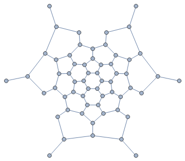
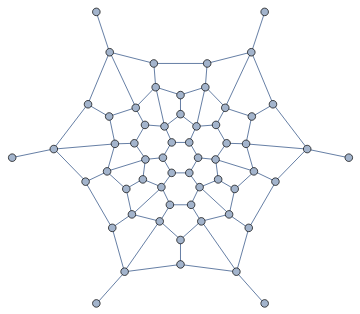
The connections we get this way are not the same as the original graph, but at least in the middle of the point set, the connections are reconstructed well.
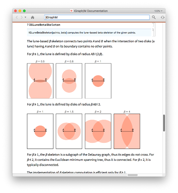
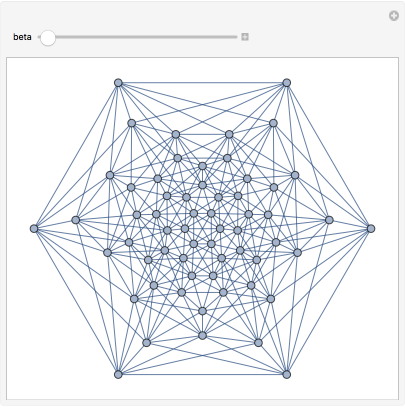
β-skeletons are proximity graphs that interpolate smoothly between the two graphs above, and beyond.
In[]:=
Manipulate[IGLuneBetaSkeleton[pts,beta],{beta,0.5,3}]
Out[]=
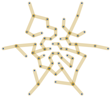
Let us construct a random maze from the Gabriel graph of these points by taking a random spanning tree.
In[]:=
With[{gg=IGGabrielGraph[pts]},IGRandomSpanningTree[gg,VertexCoordinatesGraphEmbedding[gg],GraphStyle"ThickEdge"]]
Out[]=
An exact definition of all of these proximity graphs used above is found in the IGraph/M documentation. Open it to see many more functions with many more examples by evaluating:
In[]:=
IGDocumentation[]