Non-trivial homotopies of arbitrary hypergraphs and their solitons
by Vladyslav Kuchkin
Forschungszentrum Jülich, RWTH Aachen
by Vladyslav Kuchkin
Forschungszentrum Jülich, RWTH Aachen
Topological solitons (e.g. skyrmions) that exist in different branches of physics can effectively be described as cycle subgraphs of a hypergraph in the Wolfram model. The aim of this research is to develop a method to search for such cycles. As it turned out, the distribution of lengths of optimized cycles for a given graph contains important features about graph topology even if not all cycles are taken into account. The technique is similar to Monte-Carlo methods in physics and allows one to get reasonable results in graph exploration too. For the hypergraphs that contain a subgraph with non-trivial topology, the next step will be to study the evolution of the hypergraph under diverse rules and check the behaviour of the subgraph. The physically realistic cases correspond to the conservation of the homotopy group to which the hypergraph belongs.
Topological solitons in physics and in graph theory
Topological solitons in physics and in graph theory
Particles in modern physics often demonstrate the properties of topological solitons. They appear in experiments of inter-particle interactions that obey certain conservation laws and inspired scientists to reveal these intriguing connections. The idea that nuclei stability, or conservation of its baryonic charge, is akin to topological stability arises in Skyrm’s original paper [1]. Despite the fact that such a point of view is not very popular in modern high-energy physics, the main idea has been found to be useful in other branches of science. Magnetic solitons (skyrmions) that exist in chiral magnets and present well-localized whirls in ferromagnetic background can serve as a good example. In the continuum field theory, skyrmions are topological solitons that belong to homotopy group. At the same time they live on the discrete lattice of magnetic material and due to this, it might be more reasonable to look at skyrmions from the side of discrete homotopy groups. The Wolfram model (WM) seems to be promising from this perspective because it considers a very general type of objects -- hypergraphs -- which additionally possess discrete topological properties [2]. Cycles of graphs in the WM may serve as analogues of the topological solitons in physics may serve . In this project, I concentrate mostly on S1 and S2 cycles in graphs [3]. 
 S1 cycles represent one-dimensional loops that may contract into a point (see sphere) or may remain of finite size (see torus) depending on the graph topology -- trivial or non-trivial. Due to this, finding S1 cycles of the given graph is important from the point of view of the determination of its topology, which finally helps distinguish graphs of physics interest. S2 cycles are discrete analogues for two-dimensional surfaces (see sphere and torus). Finding such cycles is the same as figuring out polyhedral embedding for an arbitrary graph, which is an NP-complete problem, although a weak form of S2 -- so-called cellular embedding -- can be solved in linear time. The results presented below cover the following topics: 1) searching for S1 cycles on a square grid -- non-directed graph, 2) ways to generalize the approach to the hypergraph case, 3) exploring S2 cycles on some graphs.
π
2
Exploring S1 cycles of a graph as an optimization problem
Exploring S1 cycles of a graph as an optimization problem
For non-directed graphs, representing natural discretizations of arbitrary manifolds, it is easy to find all its cycles using the Wolfram Language (WL) function FindCycle. At the same time, the graphs of the most interest in WM are usually big and the brute force algorithm of considering all possible cycles does not seem to be effective. This problem can be solved by exploring only some subset of all cycles which are chosen randomly, since the statistical information of this subset often already contains the needed information about topological properties of the entire graph. From the physics perspective, such an approach is akin to Monte-Carlo methods [4]. To make the sampling more effective one can perform additional length optimization for every cycle from the subset. The technique for how this optimization can be accomplished is presented below.
2D square grid case
2D square grid case
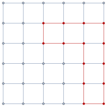
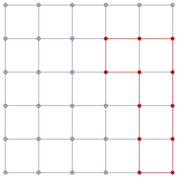
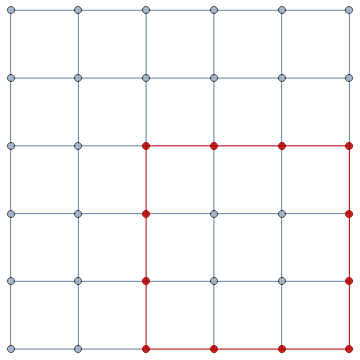
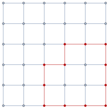
Let us consider a 2D grid graph (left); calling the function FindCycle allows us to get some cycle (right):The cycle that FindCycle returns obviously can be optimized. As it turned out, in most cases it is enough to consider two simple rules. The first one is in removing three edges of a cycle and adding a new one: This one rule is not enough because it can not optimize rectangular graphs; due to this I also add the rule that inverts the corner:The algorithm that combines these two rules allows us to optimize lengths for a cycle on square grid graphs.


-->
-->
Examples
Examples
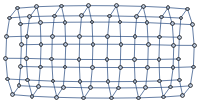
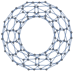
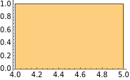
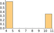
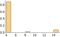
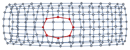
In addition to a 2D grid (left), the algorithm is applicable to different surface-like graphs (cylinder, cylinder with a hole, torus) that are shown below:, ,, .Considering subsets of cycles for these graphs and performing optimization for each cycle, it is informative to look at the distribution of the lengths of optimized cycles. Using the WL function Histogram, one can visualize these distributions presented as probability densities:, , The first spike on all histograms corresponds to a trivial cycle that for these particular cases coincides with the tessellation size -- 4 -- and can be contracted into a point. The 2D grid is topologically trivial because it has only cycles of this length. In the case of the cylinder, all nontrivial cycles have a length of 10. For the cylinder with a hole, and for the torus, there are two types of nontrivial cycles of length 8 and 14, respectively. , ,, . Additional spikes on the torus histogram do not have topological meaning and can disappear after performing more optimization steps. As we can see, even such a simple algorithm can give some useful information about graphs. Nevertheless, it has some limitations. For instance, it cannot optimize circle-like cycles. In its current form, the algorithm works only with square discretized surfaces and may fail if the graph has a large number of regions with some other tessellation. These problems can be solved and are subjects for further algorithm improvement. In the next section I consider the applicability of the algorithm for hypergraphs cases, which are the main object to study in WM.

,


S1 cycles on hypergraphs
S1 cycles on hypergraphs
The case of hypergraphs is more general due to the presence of hyperedges instead of edges, and can be thought of as a generalization of a directed graph. Although the algorithm discussed above is developed for non-directed graphs, it can be generalized straightforwardly.
Mapping between hypergraph and graph
Mapping between hypergraph and graph
The ResourseFunction HypergraphToGraph is useful because it performs the corresponding mapping between graphs while preserving some property of the hypergraph. Although in its standard implementation it creates graphs with a large number of edges, for my particular project, I have modified the use of the HypergraphToGraph function as is shown below:
In[]:=
<<SetReplace`r={{x,x,y},{x,z,u}}{{u,u,z},{y,v,z},{y,v,z}};hg=WolframModel[r,{{1,1,1},{1,1,1}},100,"FinalState"];g1=ResourceFunction["HypergraphToGraph"][hg];g2=ResourceFunction["HypergraphToGraph"][Flatten[If[Length[#]<3,{#},Partition[#,2,1]]&/@hg,1]];g3=Flatten[List[EdgeList[g2][[#,1]]EdgeList[g2][[#,2]]]&/@Range[Length[EdgeList[g2]]]];HypergraphPlot[hg]g1g2Graph[g3]
Out[]=
Out[]=
Out[]=
Out[]=
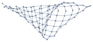
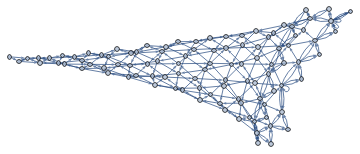
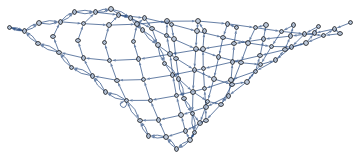
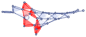
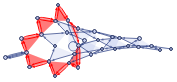
The first graph is the hypergraph (hg) from the Notable Universe Models list, the second one (g1) is its mapping obtained via the HypergraphToGraph function, the third is my modification mapping (g2) and the fourth is its non-directed version (g3).The final non-directed graph is simple to analyze with the algorithm shown above, although some information about its cycles may not be of interest from the point of view of the original hypergraph. Due to this an additional check has to be performed to figure out whether the cycle of such a non-directed graph corresponds to some cycle of the hypergraph.
Inflation-like soliton
Inflation-like soliton
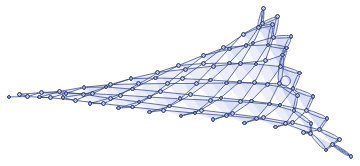
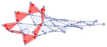
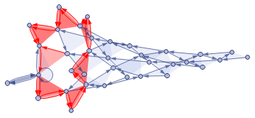
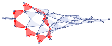
In the case of the hypergraph shown above, the S1 cycle on its growing part represents the inflation-like soliton. It can be easily found for projection graph (g2) using FindCycle function with an additional constraint -- the sum of its vertices values has to be maximal. The graph evolution below shows how this soliton transforms while the hypergraph grows:
,

,
,
,
,
Graphs with S2 cycles
Graphs with S2 cycles
Since polyhedral embedding is an NP-complete problem, it is reasonable to use less precise methods that will be more computationally economical and at the same time be able to catch some useful information regarding the presence of non-trivial S2 cycles in the graph. Intuitively it is clear that the presence of an S2 cycle leads to the presence of a gigantic number of S1 cycles in the graph, though many of them are contractable. The straightforward exploration of all such S1 cycles again does not seem to be reasonable. As it turns out, the algorithm used above for optimizing S1 cycles can give certain hints about whether a graph can have S2 cycles. As has been mentioned above, the algorithm will not work properly for circular cycles, but at the same time, there are graphs containing S2 cycles for which having a big number of such non-optimized S1 cycles can serve as good evidence of the presence of a higher homotopy group.
Sphere
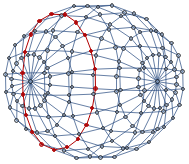
Sphere
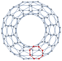
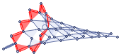
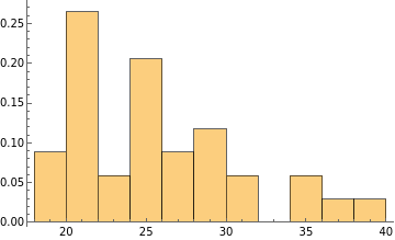
An example of the S2 cycle is the graph obtained as a discretization of a sphere. The circular S1 cycle that can not be more optimized using the algorithm above is shown in red: Excluding trivial cycles of size 4 and 3 (near sphere poles), the distribution of optimized S1 cycle lengths is:
Torus with a sphere
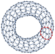
Torus with a sphere
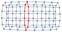
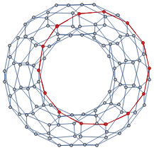
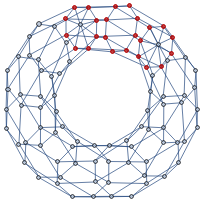
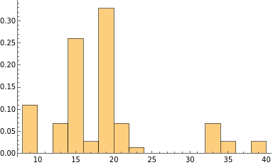
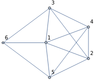
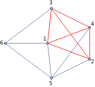
Adding two additional vertices to the torus graph leads to new S2 cycles appearing in it. The vertices that belong to the smallest S2 cycle are shown in red: Again excluding S1 cycles of trivial size, the distribution of the lengths has the form: It is interesting that in both cases (sphere and torus with a sphere), the calculated histograms contain many additional cycles that may be related to the presence of S2 cycles in the initial graph. The connection between S1 and S2 cycles is direct. Assuming that the graph contains an S2 cycle means that the set of edges of S2 can be presented as a non-intersecting union of S1 cycles of the graph where every edge of an S1 cycle appears in exactly two sets. The example below demonstrates how it works. For the graph hg = {12,13,14,15, 2 3, 24,25, 34,36, 45,56, 61} (left), one can find an S2 cycle {12, 2 3, 13, 34, 24,14} (right) that is equivalent to the union {12, 2 3, 31} ⋃ {23, 34, 42} ⋃ {12, 24, 41} ⋃ {13, 34, 41}: Therefore, analyzing S1 cycles of minimal length allows reconstruction of the S2 cycle if the graph contains one. The generalization of this definition of S2 for the case of directed graphs and hypergraphs has to take into account the edge directedness when constructing the non-intersecting union.
Concluding remarks
Concluding remarks
In this project, I have studied S1 and S2 cycles in non-directed graphs and their relation to topological solitons in physics. It has been shown that for the graph with square tessellation, the length optimization algorithm of the S1 cycle can be effectively used to determine the presence of non-trivial S1 cycles and even give some hints regarding presence of S2 cycles. The method I use allows one to find the graph homotopy group by analyzing optimized length distribution histograms, taking into account a randomly chosen subset of S1 cycles. The algorithm has been tested for graphs with square tessellation and requires additional improvement for working with graphs of arbitrary tessellation. Additionally, the further development of the project can be done in a few independent directions: 1) Study of graphs and hypergraphs belonging to higher homotopy groups. 2) Developing algorithms for effective searching of S2 and higher order cycles in graphs. 3) Exploring the connection between graphs with non-trivial topology and topological solitons in physics.
Complete project work
Complete project work
Keywords
Keywords
◼
Topological soliton
◼
Graph homotopy
Acknowledgment
Acknowledgment
I would like to acknowledge Stephen Wolfram for defining for me this project, Sam Whittington and Jonathan Gorard for supervision work, Max Piskunov, Carlos Muñoz and Hatem Elshatlawy for useful advice and help concerning Wolfram Language.
References
References
◼
Skyrme T.H.R. A Non-Linear Field Theory, Proc. R. Soc. Lond. A 260, 127 (1961).
◼
Wolfram S. A Class of Models with the Potential to Represent Fundamental Physics (2020). ArXiv:2004.08210 [Gr-Qc, Physics:Hep-Th, Physics:Math-Ph]. http://arxiv.org/abs/2004.08210
◼
Tucker, Thomas W., Gross, Jonathan L. Topological Graph Theory. United States: Dover Publications, 2001.
◼
David P. Landau and Kurt Binder. A Guide to Monte Carlo Simulations inStatistical Physics. Cambridge University Press, 4 edition, 2014.