The Quantum Stochastic Master Equation (SME) describes the evolution of an open quantum system interacting with its environment in a probabilistic manner. It extends the Lindblad master equation by incorporating stochastic noise, often modeled using quantum Wiener or Poisson processes. QSMEs are crucial for understanding decoherence, quantum measurement dynamics, and feedback control in quantum information processing. Implementation is used from: Pierre Rouchon, Jason F. Ralph (2015), Efficient Quantum Filtering for Quantum Feedback Control. Phys. Rev. A91, 012118. https://doi.org/10.1103/PhysRevA.91.012118
Dynamical equation of the quantum system:
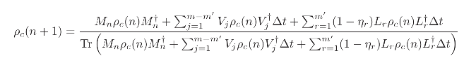
ρ=t-i[H,ρ]+ρ-,ρ+ρ-,ρ+ρ+ρ-Trρ+ρρ
∑
i
Γ
i
V
i
†
V
i
1
2
†
V
i
V
i
∑
i
γ
i
L
i
†
L
i
1
2
†
L
i
L
i
∑
i
η
i
w
i
γ
i
L
i
†
L
i
L
i
†
L
i
There are jump/Lindblad operators due to the environment, denoted by , that contribute only as decoherence term in the dynamical equation (deterministic) with the decoherence rate .
There are jump/Lindblad operators due to the monitoring of the system (with a corresponding readout), denoted by, that contribute as decoherence terms and also stochastic terms in the dynamical equation, with the decoherence rate of and the measurement channel efficiency of . Their corresponding output signal reads as
V
i
Γ
i
There are jump/Lindblad operators due to the monitoring of the system (with a corresponding readout), denoted by
L
i
γ
i
η
i
=tTrρ++
R
j
η
i
L
i
†
L
i
w
i
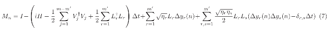
We have implemented the efficient numerical scheme proposed in this paper: https://arxiv.org/pdf/1410.5345
The main function for simulation is the following one:
The main function for simulation is the following one:
[,H,L,η,V,δt,
ρ
0
t
f
The function for manual evolution, with ρ the initial state,
H
L
V
t
f
We call it manual evolution because we do not use numerical features of Mathematica such as NDSolve or ItoProcess. The main reason for that is we were not able to using those functionalities while preserving important features of a Bloch sphere dynamics.
The readout currents are sowed in .
ℒ[ρ]=-i[Ωσx,ρ]+γD[σz] and γ >> Ω
ℒ[ρ]=-i[,ρ]+γD[]
Ωσ
x
σ
z
Hamiltonian, jump operators and damping rates:
ℒ[ρ]=-i[,ρ]+γD[]
Ωσ
x
σ
z
In[]:=
SeedRandom[1];Ω=1.0;H=ΩQuantumOperator["X"];
Jump operators and damping rates (note they are List):
In[]:=
γs={2.0};Ls={QuantumOperator["Z"]};
Time increment and final time:
In[]:=
δt=0.005;tf=20.;
Initial state:
In[]:=
ρ0=QuantumState["0"];
Solve the Lindblad master equation for the density matrix: ρ=-i[H,ρ]+ρ-,ρ
∂
t
∑
i
γ
i
L
i
†
L
i
1
2
†
L
i
L
i
In[]:=
ρt=QuantumEvolve[H,Ls->γs,ρ0,{t,0,tf}]
Out[]=
In[]:=
Plot[Evaluate@Re@ρt[t]["BlochVector"],{t,0,tf},PlotRange->All]
Out[]=
In[]:=
trajectory=ρ0,H,
γs
Ls,δt,tf;//AbsoluteTimingOut[]=
{0.115558,Null}
Check if any un-physical state:
In[]:=
PositiveSemidefiniteMatrixQ/@trajectory//Tally
Out[]=
{{True,4001}}
In[]:=
bloch=Table[Re@Tr[#.PauliMatrix[i]],{i,3}]&/@trajectory;
In[]:=
ListLinePlot[Transpose[bloch]]
Out[]=
For each trajectory, find Bloch vector:
In[]:=
Show[QuantumState["UniformMixture"]["BlochPlot"],ListLinePlot3D[bloch]]
Out[]=

Compare stochastic averaged trajectory with Lindbladian for 200 realizations (they must match):
In[]:=
Module{trjs,bloch,average,tf},tf=5;trjs=Tableρ0,H,
γs
Ls,δt,tf,200;bloch=Map[Table[Re@Tr[#.PauliMatrix[i]],{i,3}]&]/@trjs;average=Table[Re[Evaluate@ρt[t]["BlochVector"]],{t,0,tf,δt}]//Transpose;Table[ListLinePlot[{average[[i]],Mean[(Transpose/@bloch)[[All,i,All]]]},ImageSize->200],{i,3}]Out[]=
,

,
ℒ[ρ]=-i[Ωσx,ρ]+γD[σz] and γ << Ω
ℒ[ρ]=-i[,ρ]+γD[]
Ωσ
x
σ
z
Hamiltonian, jump operators and damping rates:
ℒ[ρ]=-i[,ρ]+γD[]
Ωσ
x
σ
z
In[]:=
SeedRandom[1];Ω=1.0;H=ΩQuantumOperator["X"];
Jump operators and damping rates (note they are List):
In[]:=
γs={.1};Ls={QuantumOperator["Z"]};
Time increment and final time:
In[]:=
δt=0.005;tf=20.;
Initial state:
In[]:=
ρ0=QuantumState["0"];
Solve the Lindblad master equation for the density matrix: ρ=-i[H,ρ]+ρ-,ρ
∂
t
∑
i
γ
i
L
i
†
L
i
1
2
†
L
i
L
i
In[]:=
ρt=QuantumEvolve[H,Ls->γs,ρ0,{t,0,tf}]
Out[]=
Plot the evolution:
In[]:=
Plot[Evaluate@Re@ρt[t]["BlochVector"],{t,0,tf},PlotRange->All]
Out[]=
In[]:=
trajectory=ρ0,H,
γs
Ls,δt,tf;//AbsoluteTimingOut[]=
{0.116894,Null}
Check if any un-physical state:
In[]:=
PositiveSemidefiniteMatrixQ/@trajectory//Tally
Out[]=
{{True,4001}}
Bloch vector evolution
In[]:=
bloch=Table[Re@Tr[#.PauliMatrix[i]],{i,3}]&/@trajectory;
Visualize them:
In[]:=
ListLinePlot[Transpose[bloch]]
Out[]=
Compare stochastic averaged trajectory with Lindbladian for 200 realizations (they must match) :
In[]:=
Module{trjs,bloch,average,tf},tf=20;trjs=Tableρ0,H,
γs
Ls,δt,tf,200;bloch=Map[Table[Re@Tr[#.PauliMatrix[i]],{i,3}]&]/@trjs;average=Table[Re[Evaluate@ρt[t]["BlochVector"]],{t,0,tf,δt}]//Transpose;Table[ListLinePlot[{average[[i]],Mean[(Transpose/@bloch)[[All,i,All]]]},ImageSize->200],{i,3}]Out[]=
,
,
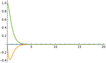
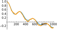
Diffusion for spontaneous emission
Diffusion for spontaneous emission
Hamiltonian, jump operators and damping rates:
In[]:=
SeedRandom[1];Δ=1.;Ω=2.;H=1/2(ΩQuantumOperator["X"]+ΔQuantumOperator["Z"]);
Jump operators and damping rates (note they are List):
In[]:=
γs={.2};Ls={QuantumOperator["J-"]};
Time increment and final time:
In[]:=
δt=0.01;tf=10.;
Initial state:
In[]:=
ρ0=QuantumState["+"];
Solve the Lindblad master equation for the density matrix: ρ=-i[H,ρ]+ρ-,ρ
∂
t
∑
i
γ
i
L
i
†
L
i
1
2
†
L
i
L
i
In[]:=
ρt=QuantumEvolve[H,Ls->γs,ρ0,{t,0,tf}]
Out[]=
Plot the evolution:
In[]:=
Plot[Evaluate@Re@ρt[t]["BlochVector"],{t,0,tf},PlotRange->All]
Out[]=
In[]:=
trajectory=Tableρ0,H,
γs
Ls,δt,tf,200;//AbsoluteTimingOut[]=
{6.77819,Null}
Check if any un-physical state:
In[]:=
Map[PositiveSemidefiniteMatrixQ]/@trajectory//Flatten//Tally
Out[]=
{{True,200200}}
In[]:=
bloch=Map[Table[Re@Tr[#.PauliMatrix[i]],{i,3}]&]/@trajectory;
In[]:=
ListLinePlot[Transpose[bloch[[1]]]]
Out[]=
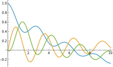
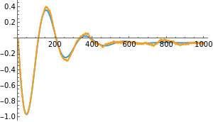
Compare stochastic averaged trajectory with Lindbladian for 200 realizations (they must match) :
In[]:=
Module[{average},average=Table[Re[Evaluate@ρt[t]["BlochVector"]],{t,0,tf,δt}]//Transpose;Table[ListLinePlot[{average[[i]],Mean[(Transpose/@bloch)[[All,i,All]]]},ImageSize->200],{i,3}]]
Out[]=
,
,
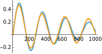
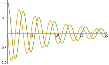
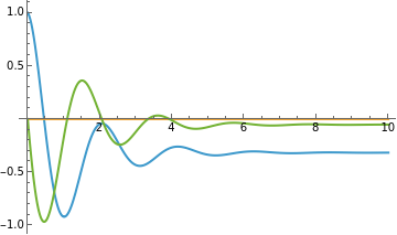
Reproducing Fig. 4.6 of Wiseman and Milburn
Reproducing Fig. 4.6 of Wiseman and Milburn
Exp #1
Exp #1
Hamiltonian, jump operators and damping rates:
In[]:=
SeedRandom[1];Δ=0;Ω=3.;H=1/2(ΩQuantumOperator["Y"]+ΔQuantumOperator["Z"]);
Jump operators and damping rates (note they are List):
In[]:=
γs={1};Ls={QuantumOperator["J-"]};
Time increment and final time:
In[]:=
δt=0.01;tf=10.;
Initial state:
In[]:=
ρ0=QuantumState["+"];
Solve the Lindblad master equation for the density matrix: ρ=-i[H,ρ]+ρ-,ρ
∂
t
∑
i
γ
i
L
i
†
L
i
1
2
†
L
i
L
i
In[]:=
ρt=QuantumEvolve[H,Ls->γs,ρ0,{t,0,tf}]
Out[]=
Plot the evolution:
In[]:=
Plot[Evaluate@Re@ρt[t]["BlochVector"],{t,0,tf},PlotRange->All,PlotLegends->{"x","y","z"}]
Out[]=
Manual simulation:
In[]:=
trajectory=ρ0,H,
γs
Ls,δt,tf;Check if any un-physical state:
In[]:=
PositiveSemidefiniteMatrixQ/@trajectory//Tally
Out[]=
{{True,1001}}
In[]:=
bloch=Table[Re@Tr[#.PauliMatrix[i]],{i,3}]&/@trajectory;
In[]:=
ListLinePlot[Transpose[bloch]]
Out[]=
In[]:=
Module{trjs,bloch,average,tf},tf=10;trjs=Tableρ0,H,
γs
Ls,δt,tf,500;bloch=Map[Table[Re@Tr[#.PauliMatrix[i]],{i,3}]&]/@trjs;average=Table[Re[Evaluate@ρt[t]["BlochVector"]],{t,0,tf,δt}]//Transpose;Table[ListLinePlot[{average[[i]],Mean[(Transpose/@bloch)[[All,i,All]]]},ImageSize->200,PlotRange->All],{i,3}]Out[]=
,
,

In[]:=
ListLinePlot[Transpose[{ArcTan[#1,#2],#3}&@@@bloch],PlotLegends->{"ϕ","cos[θ]"}]
Out[]=
In[]:=
Show[QuantumState["UniformMixture"]["BlochPlot"],ListLinePlot3D[bloch]]
Out[]=

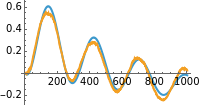
Exp #2
Exp #2
Hamiltonian, jump operators and damping rates:
In[]:=
SeedRandom[1];Δ=0;Ω=3.;H=1/2(ΩQuantumOperator["Y"]+ΔQuantumOperator["Z"]);
Jump operators and damping rates (note they are List):
In[]:=
γs={1};Ls={Exp[π/2]QuantumOperator["J-"]};
Time increment and final time:
In[]:=
δt=0.01;tf=10.;
Initial state:
In[]:=
ρ0=QuantumState["+"];
Solve the Lindblad master equation for the density matrix: ρ=-i[H,ρ]+ρ-,ρ
∂
t
∑
i
γ
i
L
i
†
L
i
1
2
†
L
i
L
i
In[]:=
ρt=QuantumEvolve[H,Ls->γs,ρ0,{t,0,tf}]
Out[]=
Plot the evolution:
In[]:=
Plot[Evaluate@Re@ρt[t]["BlochVector"],{t,0,tf},PlotRange->All]
Out[]=

Manual
In[]:=
trajectory=ρ0,H,
γs
Ls,δt,tf;Check if any un-physical state:
In[]:=
PositiveSemidefiniteMatrixQ/@trajectory//Tally
Out[]=
{{True,1001}}
In[]:=
bloch=Table[Re@Tr[#.PauliMatrix[i]],{i,3}]&/@trajectory;
In[]:=
ListLinePlot[Transpose[bloch]]
Out[]=
In[]:=
Module{trjs,bloch,average,tf},tf=10;trjs=Tableρ0,H,
γs
Ls,δt,tf,500;bloch=Map[Table[Re@Tr[#.PauliMatrix[i]],{i,3}]&]/@trjs;average=Table[Re[Evaluate@ρt[t]["BlochVector"]],{t,0,tf,δt}]//Transpose;Table[ListLinePlot[{average[[i]],Mean[(Transpose/@bloch)[[All,i,All]]]},ImageSize->300,PlotRange->All],{i,3}]Out[]=
,
,
In[]:=
ListLinePlot[Transpose[{ArcTan[#1,#2],#3}&@@@bloch],PlotLegends->{"ϕ","cos[θ]"}]
Out[]=
In[]:=
Show[QuantumState["UniformMixture"]["BlochPlot"],ListLinePlot3D[bloch]]
Out[]=

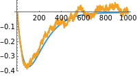
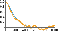
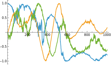
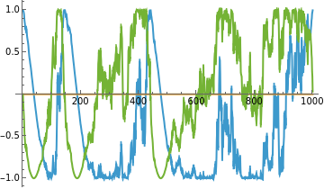
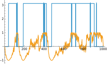
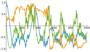
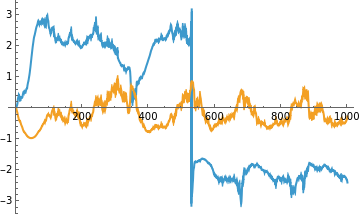
Two-point function for the stochastic homodyne current
Two-point function for the stochastic homodyne current
Hamiltonian, jump operators and damping rates:
In[]:=
SeedRandom[1];Δ=0;Ω=3.5;H=1/2(ΩQuantumOperator["Y"]+ΔQuantumOperator["Z"]);
Jump operators and damping rates (note they are List):
In[]:=
γs={.7};Ls={QuantumOperator["J-"]};
Time increment and final time:
In[]:=
δt=0.01;tf=4000.;
Initial state:
In[]:=
ρ0=QuantumState["0"];
Generate trajectory and output currents:
In[]:=
{trajectory,{Is}}=Reap@ρ0,H,
γs
Ls,δt,tf;Check if any un-physical state:
In[]:=
PositiveSemidefiniteMatrixQ/@trajectory//Tally
Out[]=
{{True,400001}}
In[]:=
ListLinePlot[Transpose[bloch]]
Out[]=
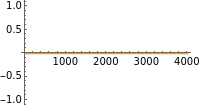
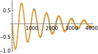
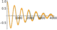
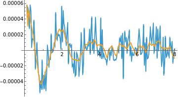
Since only one jump operator being monitored, only one current:
In[]:=
I1=Re@Transpose[Is][[1]];
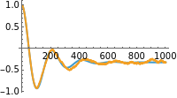
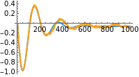
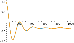
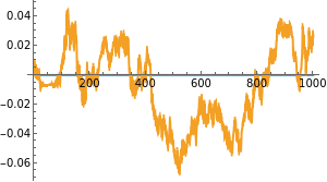
Two point correlations:
In[]:=
ℱ1=TwoPointCorrelation[Chop@Flatten@Is,Floor[8/δt],δt,4];ℱ2=TwoPointCorrelation[butterworthFilter[Chop@Flatten@Is,50,δt],Round[8/δt],δt,4];
In[]:=
ListLinePlot[{ℱ1,ℱ2}]
Out[]=
Initialization
Initialization
In[]:=
Install quantum paclet
Install quantum paclet
In[]:=
PacletInstall["https://wolfr.am/DevWQCF",ForceVersionInstall -> True]<<Wolfram`QuantumFramework`
Out[]=
PacletObject
In[]:=
Manual evolution
Manual evolution
In[]:=
ClearAll[,ℛ]

In[]:=
ℛ[ρ_,L_,δt_,δw_,η_]:=MapThread[
#3
Tr[(#1+ConjugateTranspose[#1]).ρ]δt+#2&,{L,δw,η}]In[]:=
ClearAll[][ρ_,H_,L_,η_:None,V_:None,δt_,tf_]:=Module{δw,Lmat,Vmat,Hmat,ρ0,Heff,ηm},(*η are efficiencies; if not given they are all 1*)ηm=If[MatchQ[η,None],ConstantArray[1,Length[L]],η];(*turning initial operators or states into matrices*)ρ0=ρ["Computational"]["DensityMatrix"];Lmat=#["Computational"]["Matrix"]&/@L;Vmat=#["Computational"]["Matrix"]&/@V;Hmat=H["Computational"]["Matrix"];(*given Eq.7, above, this is the term containing everything that is not random*)Heff=IdentityMatrix[2]-δt(I Hmat+.5Sum[ConjugateTranspose[l].l,{l,Lmat}]+If[MatchQ[V,None],0,.5Sum[ConjugateTranspose[l].l,{l,Vmat}]]+.5Total[ηm Table[l.l,{l,Lmat}]]);(*for each L element, generate a random process*)δw=RandomVariateNormalDistribution0,
δt
,{Length[L],Floor[tf/δt]};FoldListModule{M,st,Υ},(*for each step, create the stochastic/random terms to be added to M in Eq.7*)Υ=Total[ηm
Lmat Sow@ℛ[#1,Lmat,δt,#2,ηm]];M=Heff+.5Υ.Υ+Υ;(*evolve*)st=M.#1.ConjugateTranspose[M]+If[MatchQ[V,None],0,δt Sum[l.#1.ConjugateTranspose[l],{l,Vmat}]]+δt Sum[(1-ηm[[l]])Lmat[[l]].#1.ConjugateTranspose[Lmat[[l]]],{l,Range[Length@Lmat]}];stTr[st]&,ρ0,Transpose[δw]Two point correlation and Butterworth filter
Two point correlation and Butterworth filter
Gabriel’ s function :
In[]:=
Clear[TwoPointCorrelation];TwoPointCorrelation[data_,hmax_,dt_:None,steps_:1]:=Module{=Length@data,ave = Mean[data],vec1,M,corr},vec1 = data1;;-hmax;M = Table[data〚1+i;;-hmax+i〛,{i,1,hmax,steps}];corr=(M.vec1-);If[dt===None,corr,{dt Range[1, hmax,steps],corr}]
1
2
ave
In[]:=
Clear[butterworthFilter];butterworthFilter[data_,ωc_,dt_:1,order_:2]:=Module[{f,b},f=RecurrenceFilter[ToDiscreteTimeModel[ButterworthFilterModel[{"Lowpass",order,ωc }],dt],data];b=RecurrenceFilter[ToDiscreteTimeModel[ButterworthFilterModel[{"Lowpass",order,ωc }],dt],Reverse[data]];(f+Reverse[b])/2]
CITE THIS NOTEBOOK
CITE THIS NOTEBOOK
Quantum stochastic master equation (SME)
by Mohammad Bahrami
Wolfram Community, STAFF PICKS, January 31, 2025
https://community.wolfram.com/groups/-/m/t/3368265
by Mohammad Bahrami
Wolfram Community, STAFF PICKS, January 31, 2025
https://community.wolfram.com/groups/-/m/t/3368265