A software infrastructure for datacenter networks based on algorithms whose assumptions about causality go beyond Newtonian and Minkowski spacetime. This project is to design and verify protocols for direct (near neighbor connected) networks that can be deployed on FPGA-enabled SmartNICs to address fundamental problems in distributed systems. This leads to a system of rewriting rules that can execute in multiway application fragments ‘invisibly’ and ‘indivisibly’ in the FPGA layer one substructure.
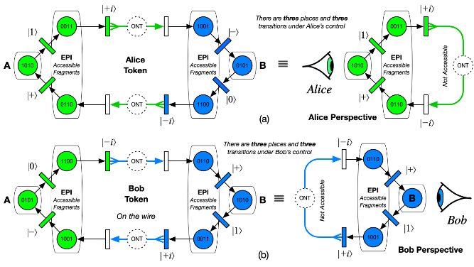
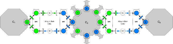
Figure 1: Dual-SAW-Petri-Spekkens Protocol
Introduction
Introduction
Maintaining liveness and synchronizing processes in Ethernet channels is a perennial challenge when packets can be dropped, reordered, duplicated or delayed. Conventional switched networks require protocol stacks and applications to use timeouts and retries to maintain liveness. This makes exactly-once semantics impossible and precipitates retry storms which lead to unbounded tail latency and transaction failure.
A single circulating (black) token with an even number of places and transitions will create a stable set of unchanging states in a Petri net. Using two tokens; one owned by Alice and one owned by Bob, will exhibit alternating ‘dynamic' liveness at places A and B. We can ‘hang’ additional information on top of this basic liveness protocol to teleport [Bennett, Bouwmeester] atomic tokens from one side of the Ethernet Link to the other, and to enable Alice and Bob to manage serializability in a distributed system of microservices based on a tree of computations.
Using colored tokens, serializability for distributed algorithms is resolved for Alice using her token, for Bob using his token, and for Charlie waiting for both tokens and deciding what order s/he wishes them to appear in. Application fragments specify ordering constraints, and Charlie's interface can compose linearizable ‘application primitives.’ By rearranging the order in which non-commutative application fragments appear, Charlie can thus coordinate serializability in a distributed system - even when the arrival order of packets appears to conflict, because (within a certain memory range) Charlie can ‘reverse time’ for the packets on local links and reorder the events to appear in a different order to match application constraints. The model generalizes to any number of different color tokens or any number of stages in a chain, tree or graph.
Alice controls serializability from her perspective, by using her Petri token, same for Bob, using his token. When the ordering of events needs to be resolved for an algorithm, cell-agents wait for all the tokens necessary to resolve the uncertainty. Do we want Alice's events to occur before Bob's, or Bob's before Alice's, or does Carol declare (from her perspective) the order for them? An easy constraint for applications to specify. This provides a deterministic primitive which the software layers above can request, related to application consistency constraints.
Ethernet
Ethernet
Ethernet is ubiquitous in modern datacenters. We define a metaphor for a substructure/superstructure (skyscraper model) with a conventional host processor and memory hierarchy above the ground, and the substructure below the ground managed by FPGA-enabled SmartNICs [Schweitzer]. The superstructure (steel frame, walls that 'hang' from the steel frame). The substructure (piles & reinforced concrete foundations). We emulate entanglement, the no-cloning theorem, and teleportation classically: In effect, (inside the network enclave/FPGA substructure) we ‘collapse' the network to a consistent state for distributed algorithms by allowing only those orders that are specified by the application as valid. We call this ‘discrete' superposition.
There is a rich history of highly creative engineering in the design of network protocols beginning with Bob Metcalfe's original Ethernet [6, 7]. Encoding each bit as low or high level (corresponding to whether the driver was on or off) on the wire for 'equal periods' is a 'self-clocking' scheme invented at Manchester. The exclusive-OR boolean function ⊕ of a clock and a data signal has no DC component, and is DC balanced. This means that binary information (0 or 1) is represented as transitions rather than voltage levels. This 'pairs' transitions for each binary digit transmitted, with an intrinsic clock recovery per bit period. The PARC Ethernet was Manchester. The cable was not driven or driven, on or off, leaving the cable off/undriven half the time, so that collisions could be detected. Half the time during a packet the cable would be undriven. Clock was recovered from transitions to or from driven state in the middle of each bit cell.
What's missing from a protocol perspective is a robust notion of reversibility. An important innovation in the next evolution of Ethernet protocols is being able to exploit reversibility to engineer recoverable systems. A simple perspective is to 'just use' Legacy Protocols such as TCP/IP and build reversible state machines at each end. To understand why this will always be insufficient, we need to explore what Shannon taught us about Information.
While there is always at least one transition per bit period to enable clock recovery at the receiver; this is a 'forward-in-time-only' concept. Without some kind of ‘convention’ there is no way to distinguish one event from another in time. This will come as a surprise to people who believe in an irreversible Newtonian Time, or even Minkowski's 4D Spacetime.
The key idea is to (a) provide all events with partners (‘closing the loop’ in Bob Metcalfe's language), and (b) to provide a reversible engine when something goes wrong, and either (i) to move the engine forward to completion (over a different link), or (ii) reverse the engine on both sides of the original link that failed to a point where the error "unhappened". In both cases, preserving the Shannon information pairings (in sequences of 1, 2, 4 and any multiple of 4).
Goals
Goals
1
.Use the Spekkens epistricted coding scheme to maintain liveness and integrity of the link.
2
.A pair of ports can maintain disjoint views of the epistemic state by constantly exchanging an atomic packet on the link. (Live heartbeat).
3
.Two atomic packets maintain liveness for Alice and Bob independently . Two independent atomic packets also provide some measure of event redundancy in case one of them fails or is corrupted.
4
.There are six combinations of the four ontic states where only half of the knowledge may exist . They are called an ‘elementary system’ by Spekkens.
5
.There are 6^2 = 36 product states (states resulting from the destructive effect of measurement).
6
.There are 4 != 24 entangled states which might be considered valid for liveness (but tested for disjoint consistency on each side).
7
.All other states are considered invalid, and may be the result of bit flip (or phase flip) errors in transmission or reception.
8
.There are only three ‘measurements,’ which are defined as a query on which of two potential states could be in. These are traditionally referred to as ‘observables’ - pairs of disjoint states : X, Y and Z.
9
.Because measurements irreversibly disturb the ontic state, the order in which the query on X, Y and Z occurs is important; and will result in different outcomes from the measurements.
10
.This provides a ‘handle’ which can be turned, under control of the ‘invariants’ expressed by application fragments, to reorder [14] what may be incompatible event orderings on a distributed data structure into a compatible one.
Spekkens Knowledge Balance Principle
Spekkens Knowledge Balance Principle
The Spekkens’ knowledge balance principle states that for a system which requires N bits of information to completely specify, only N bits of information may be known about the system at any time. The state of the system is called the ontic state (ONT), while the status of our (limited) knowledge about the system is called the epistemic state (EPI). By definition, We cannot know the ontic state (that would be a ‘God’s-Eye-View’ (GEV) of the mutual information in the link). However, when each side of an Ethernet Link is equipped with appropriate registers, it can know it’s half of the epistemic ‘knowledge’. Alice and Bob both have registers on their respective sides of the Ethernet Link to capture (a) the most recent bits put on the transmitter wire, and (b) the last bits received off the receiver channel. This represents four sets of EPI information, which (for an emulated pair of entangled qubits) can be treated as two vectors . The product of which can be viewed as a 4x4 matrix in the simulator, and used to ‘model’ the behavior of the link.
2
Whenever a two-phase commit operation is carried out over the link, there is a potential for link failure in the middle the four operations (send, ack, send, ack of the two-phase commit operation). By keeping track of the EPI information on both sides, we can employ mechanisms in a 3rd party to ‘reconnect’ the pieces of Shannon information that may have been lost by a simple "smash and restart" operation on the link (or dropped as the network re-routes packets).
SpekkensStates={{1,1,0,0},{0,0,1,1},{1,0,1,0},{0,1,0,1},{0,1,1,0},{1,0,0,1}};SpekkensPermutations={Cycles[{}],Cycles[{{1,2},{3,4}}],Cycles[{{1,3},{2,4}}],Cycles[{{1,4},{2,3}}]};AllPermutations=PermutationCycles/@Permutations[Range[4]];
There are 4! = 24 permutations of the potential ontic state (subtracting out the ones which do not correspond to the knowledge balance principle). There are = 36 product states (states resulting from the destructive effect of measurement) :
2
6
In[]:=
ArrayPlot[#,Mesh->True,ImageSize->50]&/@KroneckerProduct@@@Tuples[SpekkensStates,{2}]
Out[]=
,

,

,

,

,

,

,

,

,

,

,

,

,

,

,

,

,

,

,

,

,

,

,

,

,

,

,

,

,

,

,

,

,

,

,


Figure 2: The 6 x 6 =36 Epistemic States with Knowledge Balance.
Classical Entangled Links
Classical Entangled Links
We can construct various ‘alternating causality’ states which we can use to represent (classical) entanglement across the Ethernet Link. The 4 x 4 matrix is EPI information only, created from the two 4-bit registers (EPI-Received, and EPI-Transmitted) on each side of the Ethernet Link.
In[]:=
NestGraph[state|->Join[Permute[state,#]&/@SpekkensPermutations,SubsetMap[OperatorApplied[Permute][#],state,All]&/@SpekkensPermutations],TensorProduct@@@Tuples[SpekkensStates,{2}],4,VertexLabels->v_:>ArrayPlot[v,Mesh->True,ImageSize->30]]
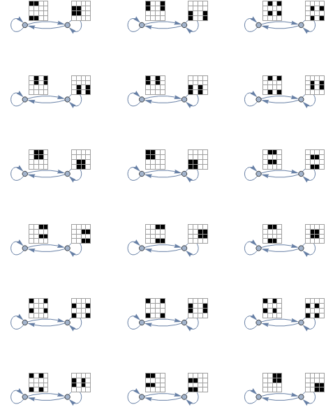
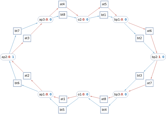
Figure 3: 18 examples of Superposition using circulating (Alternating Causality) Ethernet Frames with pure (disjoint) epistricted metadata.
Entangled State Machines
Entangled State Machines
We can construct various state machines, which will cycle through N (an even number of states) to create a classic state machine (with multiple: 1, 2, 4 or any multiple of 4) roundtrip executions. By using a Petri net, we can create two ‘interacting’ state machine across the link, with one frame owned by Alice, and one Frame owned by Bob. We assume the entangled states are continuously (alternating causality) sharing a token. The product states are ‘ready’ for measurement and can be extracted by Charlie (in the FPGAs) by doing a ‘destructive read.’
SimpleGraph@UndirectedGraph@NestGraph[state|->Join[Permute[state,#]&/@AllPermutations,SubsetMap[OperatorApplied[Permute][#],state,All]&/@AllPermutations],TensorProduct@@@Tuples[SpekkensStates,{2}],2,VertexLabels->v_:>ArrayPlot[v,Mesh->True,ImageSize->32]]
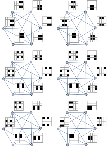
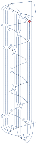
Figure 4: Six examples of state machine evolution each with 6 possibilities for epistricted (Knowledge Balanced) states used as metadata for information transfer.
Ethernet Epistricted Metadata
Ethernet Epistricted Metadata
Alice and Bob are connected on two ends of an Ethernet Link: formally, a bipartite graph which maintains a monogamous relationship through the exchange of packets. We model this system as a pair of Spekkens elementary systems, each having = 4 ontic states. When taken together we will have = 16 ontic states. A complete specification of the ontic state will therefore require 4 bits of information, whereas the knowledge balance principle requires that half (2 bits of information) may be known about the system at any time. The knowledge balance principle (KBP) continues to apply to each of the 2- bit subsystems. We note that an appropriate definition of information is Shannon information -- a surprisal. Once information has been received, it is no longer information. It is therefore appropriate to call it knowledge if we have a memory to store it in. Knowledge can be thought of as the integral of information, and information can be thought of as the derivative of knowledge.There are only 6 consistent states in the Spekkens Toy Model (STM). The disjoint pairs are shown in figure 5.
2
2
4
2
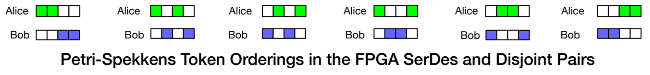
Figure 5 :
Thereare=36possibilities.Only12ofthem(6forAlice,6forBob)representconsistent/disjointpairs.
2
6
Grid Graph
Grid Graph
A set of nodes in a Grid Graph representing servers in a rack, and a row of racks. Each server has 8 ports (from the 8 lanes in a typical SmartNIC). We show 16 columns of 8 servers in Figure 6 below. The architecture is “scale independent” (Each addition of a node to the system comes with its own processor, memory, storage and network processing capability).
Base Spanning Trees
Building a Base Graph : Datacenter Racks and Server nodes
Base Spanning Trees
Building a Base Graph : Datacenter Racks and Server nodes
Building a Base Graph : Datacenter Racks and Server nodes
In[]:=
With[{g1=NearestNeighborGraph[Position[(*Anotherwayofbuildingabasegraph*)ConstantArray[1,{16,8}],1],{All,Sqrt[2]},VertexSize->1/2,VertexShapeFunction->"Octagon"]},Graph[g1,VertexStyle->Catenate[MapThread[Thread[#2->#1]&,{{Red,Green,Blue},Function[{valence},Select[VertexList[g1],VertexOutDegree[g1,#]==valence&]]/@{3,5,8}}]]]]
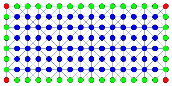
Figure 6: All nodes are identical, and have 8 ports (typically the SmartNIC has an ASIC / FPGA with 2 x 4 lanes, each with their own semi-independent SerDes (Serializer/Deserializer) running at typically 25Gbps (i.e. 8 ports - a valency of 8 for the graph algorithms).
Building a Datacenter Fabric
Building a Datacenter Fabric
Figure 6 above is a base Tree system, on top of which we provide:
1
.Recursively stacked Trees which are subsets (graph covers), for routing.
2
.Publish/Subscribe to turn a tree awareness by a child cell to an extension of that tree.
3
.Different types of stacked trees to match the infrastructure layer, e.g.:
◼
Physical Graph (the connected nodes and cables) (Valency = 8, rectangular layout to match racking and stacking of servers).
◼
Logical Graph (the sets of nodes that represent the organization (e.g. Valency 6, to match hexagonal resource allocation).
◼
Virtual Graph (arbitrary Graphs that represent applications/microservices).
Dynamic Spanning Tree Demonstration
Dynamic Spanning Tree Demonstration
In[]:=
DynamicModule[{g0=NearestNeighborGraph[Position[ConstantArray[1,{16,8}],1],{All,Sqrt[2]}],g1,selection={5,6}},Dynamic[g1=ResourceFunction["ToDirectedAcyclicGraph"][g0,{selection}];Graph[Rule[RandomChoice[VertexInComponent[g1,#,{1}]],#]&/@Complement[VertexList[g1],{selection}],VertexStyle->Flatten[MapThread[Thread[#2->#1]&,{{Red,Green,Blue},Function[{valence},Select[VertexList[g0],VertexOutDegree[g0,#]==valence&]]/@{3,5,8}}]],VertexCoordinates(#->#&/@VertexList[g1]),EdgeStyle->Directive[Gray,Arrowheads[0.015]],ImageSize->600,PerformanceGoal->"Quality",VertexShapeFunction->(EventHandler[Rectangle[#1-{1/4,1/4},#1+{1/6,1/6}],"MouseClicked":>(selection={1,1};selection=#2)]&)]]]
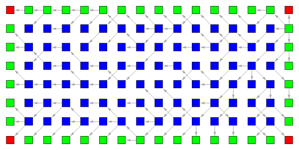
Figure 7: Dynamic Spanning Trees. Click on a node to see the spanning tree for that node.
Click on the same node again for another random spanning tree built on that same node.
Click on the same node again for another random spanning tree built on that same node.
Spanning Trees as a measure of resilience
Spanning Trees as a measure of resilience
Euler’s algorithm says there are Spanning trees (in a fully connected graph). Our’s is not fully connected (degree limited). But there is still a *very* large number of alternative spanning trees for each node. We build a spanning tree per SmartNIC, rooted on itself. Each child node has many potential spanning trees it can chose from and inform its parent nodes of its local decision, and propagate its DAG structure to its child nodes. Once a spanning tree has been built, any broken link can be healed around locally to form another spanning tree -- representing additional resilience. Euler’s formula represents a full mesh, which one would think would be the ultimate resilience, but there are problems: (1) A full mesh can never be scalable, because every time you add a new node, each existing node must increment its valency; and (2) the complexity burden of logical link state management now falls on every cell instead of being distributed throughout the tree as local-observer-view (LOV) information only.
~
N-2
N
In[]:=
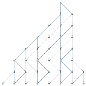
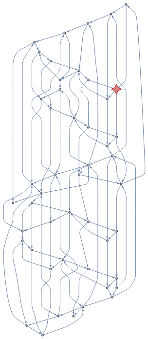
With[{minDistanceGraph=ResourceFunction["ToDirectedAcyclicGraph"][NearestNeighborGraph[Position[ConstantArray[1,{16,8}],1],{All,Sqrt[2]}],{{6,5}}]},Labeled[minDistanceGraph,Text@Row[{N[Times@@DeleteCases[VertexInDegree[minDistanceGraph,#]&/@VertexList[minDistanceGraph],0]],"Alternative Trees"},Spacer[5]]]]
Out[]=
4.64442× 45 10 |
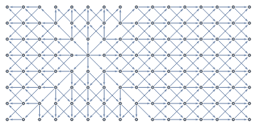
Figure 8: There are a great many alternative spanning trees ) possible with this combination of Breadth First and Depth First spanning tree building and healing.
(
45
10
Quantum Teleportation
Quantum Teleportation
“An unknown quantum state ]P) can be disassembled into, then later reconstructed from, purely classical information and purely nonclassical Einstein-Podolsky-Rosen (EPR) correlations. To do so the sender, Alice and the receiver, Bob, must pre-arrange the sharing of an EPR-correlated pair of particles. Alice makes a joint measurement on her EPR particle and the unknown quantum system, and sends Bob the classical result of this measurement. Knowing this, Bob can convert the state of his EPR particle into an exact replica of the unknown state ]P) which Alice destroyed.” [Bennet et al]
“Quantum teleportation allows for the reliable transfer of quantum information between distant nodes, even in the presence of highly lossy network connections.” [Selby]
The intuition is as follows - While the link is working correctly, we have local (link metadata) to tell us if the link is still ‘in-sync’ and both sides will know (with alternating causality) that the link is live, and that their last piece of information got through OK. If the link fails, we are only concerned if it fails in the middle of a two phase commit operation. If ‘sync’ is lost, then both sides will know, and will rendezvous through another (3rd party node) to ‘reverse’ the exchange of information on both sides of the broken link, such that the Shannon information is not lost. This will typically be done after a healing operation on the spanning tree after a link or node failure.
One Token Petri Net
One Token Petri Net
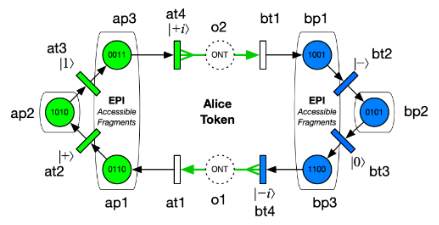
Petri net of Alice and Bob SAW-Petri-Spekkens Protocol
Petri net of Alice and Bob SAW-Petri-Spekkens Protocol
net=StylizePetriNet@PetriNet{ap2->{1,0},bp2->{0,1},ap1->{},ap3->{},bp1->{},bp3->{},o1->{},o2->{}},(*Placesandinitialcolortokens*)ap1at2,at2ap2,ap2at3,at3ap3,ap3at4,at4o2,o2bt1,bt1bp1,bp1bt2,bt2bp2,bp2bt3,bt3bp3,bp3bt4,bt4o1,o1at1,at1ap1,VertexCoordinates->{ap2->{0,0},(*Alice-Start*)at3->{2,5},ap3->{4,10},at4->{10,10},o2->{16,10},bt1->{22,10},bp1->{28,10},bt2->{30,5},bp2->{32,0},(*Bob-Center*)bt3->{30,-5},bp3->{28,-10},bt4->{22,-10},o1->{16,-10},at1->{10,-10},ap1->{4,-10},at2->{2,-5}}
{1,0}
{1,0}
{1,0}
{1,0}
{1,0}
{1,0}
{1,0}
{1,0}
{0,1}
{0,1}
{0,1}
{0,1}
{0,1}
{1,0}
{1,0}
{0,1}
Out[]=
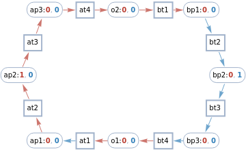
We now have a Petri net that corresponds to the picture, with the ontic states (o1) and (o2) surrounded by transitions in and out.
In[]:=
spek=<|ap2->{{1,0,1,0},{0,1,0,1}},ap1->{{0,1,1,0},{1,0,0,1}},ap3->{{0,0,1,1},{1,1,0,0}},o1->{{0,0,1,1},{1,1,0,0}},bp2->{{0,1,0,1},{1,0,1,0}},bp1->{{1,0,0,1},{0,1,1,0}},bp3->{{1,1,0,0},{0,0,1,1}},o2->{{1,1,0,0},{0,0,1,1}}|>;getSpekState[net_,places_:All]:=Total@KeyValueMap[spek[#1]#2&,PetriNetTokens[net][[Replace[places,l_List:>Key/@l]]]]getAliceState[net_]:=getSpekState[net,{ap1,ap2,ap3(*,o1*)}]getBobState[net_]:=getSpekState[net,{bp1,bp2,bp3(*,o2*)}]
Multiway execution
Multiway execution
In[]:=
NestGraph[net|->PetriNetRun[net,#]&/@PetriNetValidTransitions[net],{net},7,VertexLabels->v_:>Placed[StylizePetriNet[v,ImageSize->400,PlotLabel->Row[{Labeled[getAliceState[v],"Alice"]," + ",Labeled[getBobState[v],"Bob"]}]],Tooltip]]
Out[]=
net=StylizePetriNet@PetriNet{ap2{0,1},bp2{1,0},ap1{},ap3{},bp1{},bp3{},o1{},o2{}}(*Places*),ap1at2,at2ap2,ap1bt6,bt6ap2,ap2at3,at3ap3,ap2bt7,bt7ap3,ap3bt8,bt8o2,o2at5,at5bp1,bp1bt2,bt2bp2,bp1at6,at6bp2,bp2bt3,bt3bp3,bp2at7,at7bp3,bp3at8,at8o1,o1at1,o1bt5,bt5ap1,at1ap1,at4o2,o2bt1,bt1bp1,ap3at4,bp3bt4,bt4o1(*Transitions*),VertexCoordinates{ap2{0,0},bp2{16,0},ap1{4,-4},ap3{4,4},bp1{12,4},bp3{12,-4},at2{2,-2},o2{8,4},at3{2,2},bt2{14,2},o1{8,-4},bt3{14,-2}}(*AstaticpicureofthePetrinet.WithtwoseparatetransitionsfortheAandBtokensinoneframecircculatinginthelink*)
{1,0}
{1,0}
{0,1}
{0,1}
{1,0}
{1,0}
{0,1}
{0,1}
{0,1}
{0,1}
{1,0}
{1,0}
{0,1}
{0,1}
{1,0}
{1,0}
{0,1}
{0,1}
{1,0}
{1,0}
{1,0}
{1,0}
{1,0}
{0,1}
{0,1}
{1,0}
{1,0}
{0,1}
{0,1}
{1,0}
{0,1}
{0,1}
Out[]=
onticMultiway=SimpleGraph@VertexReplace[NestGraph[net|->PetriNetRun[net,#]&/@PetriNetValidTransitions[net],{net},14,VertexLabels->v_:>Placed[StylizePetriNet[v,ImageSize->400,PlotLabel->Row[{Labeled[getAliceState[v],"Alice"]," + ",Labeled[getBobState[v],"Bob"]}]],Tooltip],GraphLayout->"LayeredDigraphEmbedding",GraphHighlight->net,GraphHighlightStyle->"VertexConcaveDiamond",VertexSize->net->1],v_:>PetriNetTokens[v]](*ThisisapicutreofthemultiwayeveolutionofthePetrinet*)(*Amanipulatecouldbenice,withacheckboxtohave[a]AnAlicetoken,and[b]aBobToken].Ifwerunitwithonetoken,itshouldsimpify.Butthenitwouldn'thaveitsinterestingPetriinteractions*)
Out[]=
In[]:=
epiMultiway=SimpleGraph@VertexReplace[NestGraph[net|->PetriNetRun[net,#]&/@PetriNetValidTransitions[net],{net},12,VertexLabels->v_:>Placed[StylizePetriNet[v,ImageSize->400,PlotLabel->Row[{Labeled[getAliceState[v],"Alice"]," + ",Labeled[getBobState[v],"Bob"]}]],Tooltip],GraphLayout->"LayeredDigraphEmbedding",GraphHighlight->net,GraphHighlightStyle->"VertexConcaveDiamond",VertexSize->net->1],v_:><|"Alice"->getAliceState[v],"Bob"->getBobState[v]|>]
Out[]=
In[]:=
IsomorphicGraphQ[onticMultiway,epiMultiway]
Out[]=
False
Extension to 3rd-party Operations
Extension to 3rd-party Operations
Alice an Bob are implicit in each Link. These are pure 2-party (bipartite) monogamous relationships. A 3rd party can be introduced only at the next (e.g. node) level. Each node has a valency of 8. Each link can independently resolve the symmetry breaking; sometimes resulting in this end of a port being Alice (a) and sometimes Bob (b). This symmetry breaking (arrow) remains stable until the link is reset.
Conclusions
Conclusions
We have shown three things (1) A Petri net model of a quantum-inspired Ethernet protocol. (2) an epistricted (Spekkens) model for EPI registers on each side of an Ethernet link, and (3) A Layer One FPGA Ethernet Mesh network, complete with base spanning trees in the FPGA substructure. We can build on this foundation in the future to include explicit application management of causal structures using Tali Beynon’s Quiver Geometry. [17]
References
References
1
.Samson Abramsky: Petri Nets, Discrete Physics, and Distributed Quantum Computation. https://www.cs.ox.ac.uk/files/381/fest.pdf
2
.3
.Robert Spekkens: Quasi-quantization: classical statistical theories with an epistemic restriction. https://arxiv.org/abs/1409.5041
4
.Robert Spekkens. In defense of the epistemic view of quantum states: a toy theory. https://arxiv.org/abs/quant-ph/0401052
5
.John H. Selby, David Schmid, Elie Wolfe, Ana Belén Sainz, Ravi Kunjwal, Robert W. Spekkens. https://arxiv.org/abs/2112.04521
6
.Robert Metcalfe. Packet Communication. MIT/LCS/TR-114. https://web.archive.org/web/20121115055132/http://publications.csail.mit.edu/lcs/pubs/pdf/MIT-LCS-TR-114.pdf
7
.Robert Metcalfe and David R. Boggs. Ethernet: DIstributed Packet Switching for Local Computer Networks. https://dl.acm.org/doi/pdf/10.1145/360248.360253
8
.Hermans, et al. Qubit teleportation between non-neighbouring nodes in a quantum network. Nature 605, 663–668 (2022). https://doi.org/10.1038/s41586-022-04697-y
9
.Scott Schweitzer. The Rise of SmartNICs. https://www.linkedin.com/pulse/rise-smartnic-scott-schweitzer-cissp
10
.Bennett, C. H. et al.. Teleporting an Unknown Quantum State via Dual Classical and Einstein-Podolsky-Rosen Channels https://journals.aps.org/prl/pdf/10.1103/PhysRevLett.70.1895
11
.Bouwmeester, D. et al. Experimental quantum teleportation. Nature 390, 575–579 (1997). https://arxiv.org/abs/1901.11004
12
.Lay Nam Chang, Djordje Minic, and Tatsu Takeuchi. Spekkens’ Toy Model, Finite Field Quantum Mechanics, and the Role of Linearity. https://arxiv.org/pdf/1903.06337.pdf
13
.A conversation between Bob Metcalfe and Stephen Wolfram at the Wolfram Summer School 2022. https://youtu.be/Vti0sCgfXsQ
14
.Paul Borrill. TIme, Clocks and the (re)ordering of events. Lamport’s Unfinished Revolution. August 2016. https://www.youtube.com/watch?v=CWF3QnfihL4&t=1947s
15
.Paul Borrill. Insights in the Nature of Time in Physics, and Implications for Computer Science. Stanford EE380. https://www.youtube.com/watch?v=SfvouFIVCmQ
16
.A conversation between Jonathan Gorard and Stephen Wolfram at the Wolfram Summer School 2022. https://youtu.be/V_n6Xt6kcFA
17
.Tali Beynon. Quiver Geometry. https://youtu.be/RTlHJ4owHZU
Acknowledgments
Acknowledgments
Special Thanks to: Jonathan Gorard, Nik Murzin, Bradley Klee, James Boyd and Stephen Wolfram for giving me the opportunity to develop this idea at the 2022 Wolfram Summer School, mentoring me in the Wolfram Language, category theory, Petri nets, Graph Theory, and many other things. Thanks also to all my fellow students who shared this experience with me and made it such an incredibly productive and enjoyable experience. Special affection and admiration for Robert Metcalfe; who I should have met decades before this summer school.
Initialization Cells (Hidden)
Initialization Cells (Hidden)