A third-order linear ordinary differential equation in general has the form , where is the unknown function and are known functions of . These equations are typically very difficult to solve explicitly, so instead, people try to at least understand their behavior through simplifications and tricks. One such trick is presented in this essay: how to convert a general 3rd order linear ODE to the (relatively) simple form via a change of variables - in other words, how to set the coefficients before and to zero. The computation is fairly nontrivial: it involves solving another ODE and taking a couple of difficult integrals; however, more often than not it is doable and thus makes a valuable addition to the mathematical toolbox.
u'''+au''+bu'+cu=f
u=u[t]
a,b,c,f
t
v'''+Zv=F
v''
v'
w''[t]=[t]w[t]
2
p
Deriving the formula
Deriving the formula
A general third-order linear ordinary differential equation has the form
u'''[t]+a[t]u''[t]+b[t]u'[t]+c[t]u[t]=f[t]
(
1
) The equation is currently written in terms of , however, we can make a change of variables and re-write it in terms of some other function . There are many ways in which a change of variables could be done. Consider the following transformation:
u[t]
v[t]
u[t]=A[t]v[ϕ[t]]
(
2
) Effectively, this change of variables replaces with and multiplies the expression by some scaling function . Substituting this into (1) yields
t
ϕ
A[t]
Av+(aA+3A'+3Aϕ'ϕ'')v+(Abϕ'+2aA'ϕ'+3ϕ'A''+aAϕ''+3A'ϕ''+Aϕ''')+(Ac+bA'+aA''+A''')v=f[t]
3
(ϕ')
3
d
3
dϕ
2
(ϕ')
2
(ϕ')
2
d
2
dϕ
dv
dϕ
(
3
) That is how the ODE is written in terms of the variables and . Effectively, it is in the same form as the initial ODE (1), the only difference being that the coefficients have changed. Here, denotes a derivative and is reserved for the time derivative. At this point, the functions and could be anything, but for the change of variables to be useful, let us try to find such and that the coefficients before v and are zero:
v
ϕ
d
dϕ
ϕ
'
A
ϕ
A
ϕ
2
d
2
dϕ
dv
dϕ
aA+3A'+3Akk'=0Abk+2aA'k+3kA''+aAk'+3A'k'+Ak''=0
2
k
2
k
(
4
) Here, is a short-hand notation for . If we solve these equations, the ODE (3) will have the desired simple form. Dividing the first equation by yields . Integrating this with respect to time, we get a[]+3Log[A]+3Log[k]=. Solving for yields
k≡ϕ'[t]
dϕ/dt
A
2
k
a+3+3=0
A'
A
k'
k
t
∫
t
1
dt
1
∼
A[t]
A=Exp-a[]
1
1
3
t
∫
t
1
dt
1
1
k
(
5
) Plugging this in to the second equation in (4), we get . The equation is nonlinear which makes it difficult to solve; however, it can be made linear by introducing
3-2=+a'-b
2
k'
k
k''
k
1
3
2
a
w[t]≡
1
k[t]
(
6
) The equation is written in terms of as
3-2=+a'-b
2
k'
k
k''
k
1
3
2
a
w
w''[t]=[t]w[t]
2
p
(
7
) Where [t]≡+. Unlike the previous equation, (7) is linear, which makes it tremendously easier to solve, both exactly and approximately. From (6), can then be computed as . The definition requires that . Coming back to the definition and requiring to be smooth, we see that the condition simply demands a one-to-one relationship between and . This is very natural because in the change of variables (2) is the “transformed time”, and it only makes sense if there is a one-to-one relationship between time and “transformed time”. Substituting this into (5) and setting =1, we get the final formula for :
2
p
2
a[t]
12
a'[t]-b
4
w[t]≡1
k[t]
k
k=
1
2
w
w[t]≡1
k[t]
k!=0
k[t]≡ϕ'[t]
ϕ[t]
k!=0
ϕ
t
ϕ
1
A[t]
A[t]=Exp-a[][t]
1
3
t
∫
t
1
dt
1
2
w
(
8
) Making equal to any other nonzero number (for instance, 2) wouldn’t really change much because it would just correspond to rescaling by some constant. Since , is the integral of :
1
A
k[t]≡ϕ'[t]
ϕ[t]
k[t]=1/
2
w
ϕ[t]=[]
t
∫
dt
1
2
w
t
1
(
9
) And this is it! The problem is solved. If we substitute , where and are given by (8) and (9), into the ODE (3), we would see that the coefficients before and are indeed zero. The ODE can be written in the form
u[t]=A[t]v[ϕ[t]]
A
ϕ
v''
v'
3
d
3
dϕ
(
10
) Where and are given by
Z
F
Z[ϕ]≡[t](4-18a[t](b[t]-[t])+9(6c[t]-3[t]+[t]))F[ϕ]=[t]f[t]
1
54
6
w
3
a[t]
′
a
′
b
′′
a
6
w
A[t]
(
11
)Code used to do the calculations
Code used to do the calculations
Computer implementation
Computer implementation
The function below executes the algorithm described above. It first computes and tries to find . If no solutions were found, it just returns the general formulas for . If one solution was found, it substitutes the formula for into (8) and (9) and outputs concrete formulas for . If multiple solutions were found, it outputs the general formulas for and gives the user the list of possible .
2
p
w[t]
ϕ,A,Z,F
w
A,ϕ,Z
ϕ,A,Z,F
w
In[]:=
ClearAll[findϕAZF];findϕAZF[a_Function, b_Function, c_Function, f_Function] := Block t, p2, w, possiblew, wIndicator, Aval , p2 = + ; possiblew = DSolve[w''[t] p2 w[t], w, t]; Which[ SameQ[Head[possiblew], DSolve], wIndicator = Evaluate[w''[t] p2 w[t]], (* if couldn't solve *) Length[possiblew] 1, w = possiblew[[1, 1, 2]]; wIndicator = Nothing, (* if found exactly one solution *) Length[possiblew] > 1, wIndicator = (w ∈ possiblew[[All, 1, 2]]) (* if found several solutions *) ]; Aval = Exp-Integrate[a[t], t] ; Simplify@ϕ Integrate, t, wIndicator, A Aval, Z (4 -18 a[t] (b[t]-[t])+9 (6 c[t]-3 [t]+[t])), F -> f[t];
2
a[t]
12
a'[t] - b[t]
4
1
3
2
w[t]
1
2
w[t]
1
54
6
w[t]
3
a[t]
′
a
′
b
′′
a
6
w[t]
Aval
In[]:=
ClearAll[getZFform];getZFform[{ϕ -> ϕval_, A -> Aval_, Z -> Zval_, F -> Fval_}] := Block[{texpr}, texpr = Solve[ϕval == ϕ, t]; Which[ SameQ[Head[texpr], Solve], Return[$Failed], Length[texpr] >= 1, texpr = texpr[[1, 1, 2]]; u[t] == Aval v[ϕ], t == texpr, Z -> Zval /. t -> texpr, F -> Fval /. t -> texpr ]];
Here is how to use this method:
1
.Get the ODE to the form ; identify the functions .
u'''[t]+a[t]u''[t]+b[t]u'[t]+c[t]u[t]=f[t]
a[t],b[t],c[t],f[t]
2
.Run findϕAZF to find .
ϕ[t],A[t],Z[t],F[t]
3
.The expressions for are going to contain two arbitrary constants. Choose values for the constants, preferably to make the expressions simpler.
ϕ[t],A[t],Z[t],F[t]
4
.Run getZFform to find and expressed in terms of .
Z
F
ϕ
Simple! Of course, this isn’t going to work with each and every ODE. Often, the program is unable to find , or invert to find , or to compute some of the integrals. In those cases, one can resort to manual tuning and computation, which would often help lift the stalemate. It is also possible to use approximate methods such as Frobenius series. This would require some work, but even then the process isn’t too laborious.
ϕ[t]
ϕ[t]
t[ϕ]
Simple example: u'''+u''+u'+u=Log[6+2t]
Simple example:
u'''+u''+u'+u=Log[6+]
2
t
The equation is very simple, which makes it a great initial example to show that the formula works. On practice we could just solve it explicitly without bothering to get it to the form, but it is just interesting to see how things would go. Step 1: We can see that the coefficients in this ODE are , and the external force is . Step 2: Run the function findAϕZF:
v'''+Zv=F
a=b=c=1
f[t]=Log[6+]
2
t
In[]:=
findϕAZF[1&,1&,1&,Function[t,Log[6+]]]
2
t
Out[]=
ϕCos+Sin,ACos+Sin,ZCos+Sin,FLog[6+]Cos+Sin
6
Sint
6
2
1
t
6
1
2
t
6
-t/3
2
1
t
6
2
t
6
20
27
6
1
t
6
2
t
6
t/3
2
t
4
1
t
6
2
t
6
Step 3: The choice of constants , is arbitrary. Let us take =1,=0:
1
2
1
2
In[]:=
%/.{C[1]1,C[2]0}
Out[]=
ϕ,A,Z,FLog[6+]
6
Tant
6
-t/3
2
Cos
t
6
20
27
6
Cos
t
6
t/3
4
Cos
t
6
2
t
Step 4: Run getZFform:
In[]:=
getZFform[%]
Out[]=
u[t]v[ϕ],,Z,F
-t/3
2
Cos
t
6
The expression contains an arbitrary constant due to the translation symmetry of trigonometric functions; can in general contain arbitrary constants. Take =0:
1
t[ϕ]
1
In[]:=
%/.C[1]->0
Out[]=
u[t]v[ϕ],t,Z,FArcTanLog6+6
-t/3
2
Cos
t
6
6
ArcTanϕ
6
20
27
3
1+
2
ϕ
6
2
3
ϕ
6
2
ArcTan
ϕ
6
2
1+
2
ϕ
6
So, the ODE can be written as
3
d
3
dϕ
160
3
(6+)
2
ϕ
2
3
ϕ
6
2
ArcTan
ϕ
6
2
(6+)
2
ϕ
If we now substitute into the original ODE , we see that it indeed holds:
u[t]=A[t]v[ϕ]
u'''[t]+u''[t]+u'[t]+u[t]=Log[6+]
2
t
In[]:=
Simplifyu'''[t]+u''[t]+u'[t]+u[t]/.u->Function[t,A[t]v[ϕ[t]]]/.ϕFunctiont,,AFunctiont,/.v'''[ϕ_]->-v[ϕ]+36ArcTanLog61+,Assumptions->{-π/2<t<π/2}
6
Tant
6
-t/3
2
Cos
t
6
160
3
(6+)
2
ϕ
2
3
ϕ
6
2
ArcTan
ϕ
6
2
(6+)
2
ϕ
Out[]=
Log[6+]
2
t
Notice that the result only makes sense for because goes to infinity at . This is one of the drawbacks of the formula: it can often introduce limitations out of nowhere.
-π/2<t<π/2
ϕ=
6
Tant
6
t=±π/2
A more complicated example: u'''+tu''+u'+u=Sin[t]
A more complicated example:
u'''+tu''+u'+u=Sin[t]
The ODE is very difficult to solve exactly, and this is one of those cases when the method presented in this essay may be of interest. The function could not be found explicitly for this ODE, and instead, an indefinite integral is returned:
u'''+tu''+u'+u=Sin[t]
ϕ[t]
In[]:=
findϕAZF[#&,1&,1&,Function[t,Sin[t]]]
Out[]=
ϕ1ParabolicCylinderD-,+ParabolicCylinderD-,t,AParabolicCylinderD-,+ParabolicCylinderD-,,Z(27+2)ParabolicCylinderD-,+ParabolicCylinderD-,,FParabolicCylinderD-,+ParabolicCylinderD-,Sin[t]
2
2
1
2
t
1/4
3
1
1
2
t
1/4
3
-
2
t
6
2
2
1
2
t
1/4
3
1
1
2
t
1/4
3
1
27
3
t
6
2
1
2
t
1/4
3
1
1
2
t
1/4
3
2
t
6
4
2
1
2
t
1/4
3
1
1
2
t
1/4
3
The integral can be evaluated approximately using methods such as Taylor series or numerically; for simplicity, the example will go with the latter option. Choose =1, =0:
1
2
In[]:=
%/.{C[1]->1,C[2]->0}
Out[]=
ϕ1t,A,Z(27+2),FSin[t]
2
ParabolicCylinderD-,
1
2
t
1/4
3
-
2
t
6
2
ParabolicCylinderD-,
1
2
t
1/4
3
1
27
3
t
6
ParabolicCylinderD-,
1
2
t
1/4
3
2
t
6
4
ParabolicCylinderD-,
1
2
t
1/4
3
Now, the equation can be written as
3
d
3
dϕ
1
27
3
t
6
ParabolicCylinderD-,
1
2
t[ϕ]
1/4
3
2
t
6
4
ParabolicCylinderD-,
1
2
t
1/4
3
The function could not be found, not to mention inverted to find . However, it’s easy to compute a numerical solution. If , then =, and =. This is a simple differential equation that can be solved numerically, or, if more accuracy is needed, using a series solution. For simplicity, this example will go with the former option:
ϕ[t]
t[ϕ]
ϕ=t
1
2
ParabolicCylinderD-,
1
2
t
1/4
3
dϕ
dt
1
2
ParabolicCylinderD-,
1
2
t
1/4
3
dt
dϕ
2
ParabolicCylinderD-,
1
2
t
1/4
3
In[]:=
myt=NDSolvet'[ϕ]==,t[0]==0,t,{ϕ,0,3}[[1,1,2]];
2
ParabolicCylinderD-,
1
2
t[ϕ]
1/4
3
In[]:=
Plot[myt[ϕ],{ϕ,0,3},AxesLabel->{"ϕ","t"}]
Out[]=
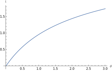
To find the functions and , we just substitute the numerical result into the formulas:
Z
F
In[]:=
Plot[#[[2]],{ϕ,0,3},AxesLabel->{"ϕ",#[[1]]},ImageSize->Medium]&/@"Z",(27+2),"F",Sin[t]/.t->myt[ϕ]
1
27
3
t
6
ParabolicCylinderD-,
1
2
t
1/4
3
2
t
6
4
ParabolicCylinderD-,
1
2
t
1/4
3
Out[]=
,
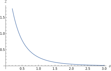
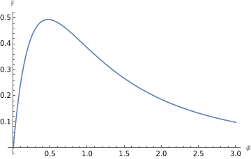
There is no closed formula for and , however, the functions can be computed to any specified accuracy. Alternatively, if a Taylor series solution for is found, it can also be substituted into and to obtain a series expansion for those. The important thing is that the ODE can be converted to the form, which paves the way for many different ways of analyzing it further. As you can see, the simplification method also works on the more difficult ODEs.
Z
F
t[ϕ]
Z
F
v'''+Zv=F