

Abstract
Abstract
In practice, due to poor data generation, there are often non-standardized headings in a spreadsheet table, and there are often multiple datasets in one single spreadsheet. Our goal was to build a function that can automatically understand a natural spreadsheet and extract tabular data so that data science algorithms can be applied without errors. For this purpose we interpreted the heads of each entry in the spreadsheet as a number and processed the resulting data as an image. For the purpose of image segmentation there are already some powerful functions in WL.
As a result we receive a list of datasets, that represent all the tables in the spreadsheet. Thanks to this function we can import the spreadsheet and immediately start working on the data without manually extracting and organizing the data.
I followed two different approaches: The first approach is image segmentation. It is described in the first section and is a good way to extract single tables from a spreadsheet but less well suited to derive clean data from a very messy table.
The second idea is to use clustering on columns of consistent datatypes. This is a complex method hat can potentially deal with very complex data structures. In this article I only lay out the basic idea.
Image Segmentation
Image Segmentation
Visualize example data (.xls files)
Visualize example data (.xls files)
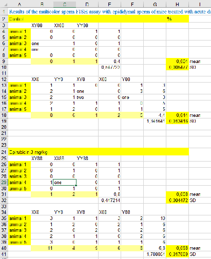
The “Import”-funcitons returns the example spreadsheet as a list of lists where all sublists are of the same length. In this case we used I labelled this list in the way that missing entries, strings and numbers are replaced by the numbers 0, 1, 2 respectively. Colorizing this labelled list returns the picture below. This kind of labelling will be necessary for data cleaning to obtain columns of only one data type.

file=Import[filepath] labelEntry[x_]:= Which[ SameQ[x, "Nothing"], 0, SameQ[Head[x],String], 1, SameQ[Head[x], Real], 2, SameQ[Head[x], DateObject], 3, SameQ[Head[x], Symbol], 4, SameQ[Head[x], Integer], 5 ]t = file/."""Nothing";labels=Map[labelEntry,t,{Length[Dimensions[t]]}];
Morphological operations on binary labeled of data
Morphological operations on binary labeled of data
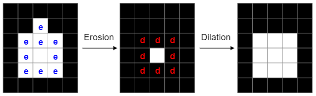
Morphological operations of erosion and dilation allow to smooth the edges of image segments: The function of erosion flips all those pixels in a binary image from the value 1 to the value 0 , that are not surrounded itself surrounded by pixels of the value 1. Dilation does the opposite: It flips the value of the pixels, that are already bordering on a pixel of the value 1, from 0 to 1. By combining these two methods I successfully reduced the tables in the data to almost rectangular shape. Source: Washington University in St.Louis, School of Engineering & Applied Science, CSE 554, Lecture 1: Binary Pictures, 2016, Slide 36 For this purpose the data is labelled binary with 0 for empty entries and 1 for entries with data. Then erosion and dilation are performed on the data. The result is displayed in the picture below. This is an effective method to delete all descriptive surroundings of the relevant data.
In[]:=
operatedOn=Dilation[Erosion[ReplaceAll[{21,31,41,51}][labels],1],1];

“Mask” to “Bounding Boxes (x_min, y_min, x_max, y_max)”
“Mask” to “Bounding Boxes (x_min, y_min, x_max, y_max)”
The third step is to extract the connected areas in the image. The WL-function “MorphologicalComponents” is very helpful with this: It labels the unconnected areas of data in the table with different numbers. The result is displayed in the image below where every area is labelled with one number.

In[]:=
connected=MorphologicalComponents[operatedOn];
To extract the colorized areas from the original data, I had to define where in the image these areas are and how big they are in each dimension. This is done via socalled bounding boxes: Using minimum and maximum values in both dimensions these boxes describe the location and size of the minimal rectangular square, that includes all entries of one label and therefore all entries of one singular table within the data.Retrieving upper and lower x- and y-values for each rectangle works in four steps: 1. I made a list of the labels in the data which is a list of integers from 1 to the number of subtables contained in the data. 2. For each of these labels I set the label itself to 1 and all other labels to 0. 3. Using the function “Position” I can create a list of all the coordinates of every entry of the number 1 in the format (x,y). 4. Using the function “MinMax” on the first and the second column of the list of positions I get the values that define the smallest possible rectangle surrounding a single table in the origianl data.
In[]:=
getSingleMask[maskLabels_, label_]:= Module[ {numLabels, complement, substitutionRule, singleMask}, numLabels = Union @ Flatten @ maskLabels; complement = Complement[numLabels, {0, label}]; substitutionRule = Sort @ Flatten[{Thread[complement Table[0, Length[complement]]], {label 1}}]; singleMask = maskLabels /. substitutionRule]getBoundingBox[singleMask_]:= Module[ {positions, xMinMax, yMinMax}, positions = Position[singleMask, 1]; yMinMax = MinMax[positions〚All, 1〛]; xMinMax = MinMax[positions〚All, 2〛]; Flatten[Transpose[{xMinMax, yMinMax}], 1]]getBoundingBoxes[maskLabels_]:= Module[ {labels}, labels = Rest[Union[Flatten[maskLabels]]]; getBoundingBox[getSingleMask[maskLabels, #]] &/@ labels]boundingBoxes=getBoundingBoxes[connected];
Return a list of single datasets
Return a list of single datasets
As a final result, the written code extracts the data within the defined boxes from the original file.
f[liste_]:=Dataset[test][liste[[2]];;liste[[4]],liste[[1]];;liste[[3]]];result=Map[f,boundingBoxes];
Out[]=
,
,
,
A different challange
A different challange
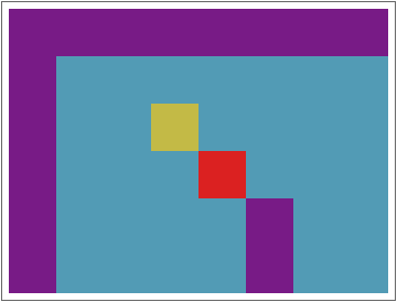
Sometimes the spreadsheet we work with is not an agglomeration of several tables but one very messy table with empty areas and areas of different datatypes. Depending on wether or not a column is a timeline, missing values can be replaced by rolling means or need to be deleted. I build an example for a very messy table and colorized the heads of the entries.
table=Import[filepath]Union[Head/@(Flatten@table)];t = table/."""Nothing"; labels=Map[labelEntry,t,{2}];rc=RandomColor[Length[labels]];colorMap=Thread[labels rc];
0,1,2,3
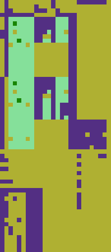
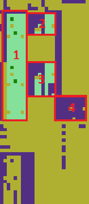
The table is widely empty (yellow). Top and bottom consist mostly of descriptive strings. But there are roughly 4 areas of valid data. Retrieving these areas with their row and column names and cleaning them would not be possible with the algorithm used thus far. The following images show the same table: In the left picture the four areas that should be extracted as subtables are marked, in the right image connected areas are coloured individually. As all four interesting subtables are colored equally, the image segmentation algorithm cannot discern them. I lay out another approach in the next chapter.

The way ahead
The way ahead
To generate datasets on which algorithms can work without errors we need to clean the data. In terms of image processing, we need rectangular areas of one color without any spots. For data cleaning we need a function that determines, wether deleting the row or the column of a missing value is preferable. One criterion could be the number of valid values, that are deleted in said row or column. Furthermore, there is the need for a “rolling means”-function, that replaces missing values in timelines with rolling means. The third idea is to combine image segmentation with the idea of clustering in chapter 2 to produce a powerful algorithm that can work on all kinds of messy spreadsheets.
Future directions: Clustering of subcolumns
Future directions: Clustering of subcolumns
How it works
How it works
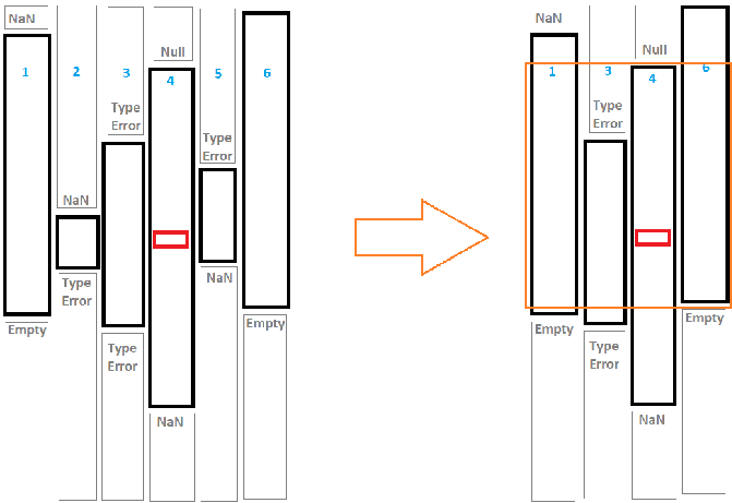
The idea is, to start with a nucleus cell (marked red in the sketch below). I retrieve the datatype of the cell and check, how far above and below the same data type goes without interruption by a NaN or another data type. I save that column (in the sketch: column 4) with its column number and upper and lower boundaries. Then I go into the neighboring columns and do the same thing. This leads to the left sketch. Now I describe every consistent column as a data point of (column number, upper end, lower end) and cluster these data points by the upper end and lower ende. Depending on the hyperparameters this will result in something like the right sketch: I get columns with roughly the same upper and lower end. I can extract these and group them together. An first draft for a code is given below.
A major advantage of this approach is, that the final tables do not need to be one connected are in the original spreadsheet but can be assembled from all columns in the spreadsheet.
A major advantage of this approach is, that the final tables do not need to be one connected are in the original spreadsheet but can be assembled from all columns in the spreadsheet.
Out[]=
The following piece of code defines a small list of lists and colors it outputs and array plot which is colored according to the head of each entry.
In[]:=
t={{"","Big","Athletic","Friendly","Trainable","Resourceful","Animal","Lucky"},{"Dog",80,20,90,90,5,100,40},{"Cat",50,40,40.,70,10,100,40},{"Rat",10,70,20,Null,80,99,40},{"Cockroach",0,80,2,20,"ninetyfive",20,40},{"Wallaby",35,52,38,47,"fourtyeight",80,40}};indexer[lst_]:=Module[{max=1,assoc=Association[],res}, Map[res=Lookup[assoc,Head[#],max]; If[res===max,assoc[Head[#]]=res; max=max+1]; res&,lst,{2} ] ]ArrayPlot[indexer[t],ColorFunction"Rainbow"];
The next piece of code defines a funciton called les (length-end-start) that returns for every entry of the table three values. These values describe the column of consistent data, the entry is in. For example: In the picture above there es one data type without interruption in column 2 from row 2 to row 6. All the entries in column 2 from row 2 to row 6 have the entry (5,6,1), describing this data column.
The last command in the code below returns an association of the following pattern: it lists for every column in the dataset all the subcolumns of consistent data with its (length-end-start)-pattern and associates it with its length.
The last command in the code below returns an association of the following pattern: it lists for every column in the dataset all the subcolumns of consistent data with its (length-end-start)-pattern and associates it with its length.
In[]:=
les[a_]:=Module[{high,low}, n=0; b=ArrayFilter[If[#[[2]]#[[1]],n=n+1,n=1]&,a,1]; c=Transpose[Reverse[MapIndexed[{#1,#2[[1]]}&,b]]]; Reverse[ArrayFilter[If[#[[2,1]]==#[[2,2]]+1 ,{n,high,low},{n=#[[2,2]],high=#[[3,2]],low=high-n}]&,c,1][[1]]] ]Transpose[Map[les,Transpose[indexer[t]]]];Map[Counts[#]&,Map[les,Transpose[indexer[t]]]]//TableForm;
In the final step I took for this approach, I create a transposed matrix of the dataset, flatten it and delete all the duplicates. This leads to the preliminary final result: All the consistent subcolumns contained in the original dataset are listed as triplets of data in the pattern of (column - first row - last row). Clustering these data triplets of the first and last row would lead to areas of consistent data in the original spreadsheet.
In[]:=
insertcolumn[{x_,y_,z_},{v_,w_}]:=Module[{},{v,z,y}]a = MapIndexed[insertcolumn,Map[les,Transpose[indexer[t]]],{2}];b=Flatten[Map[DeleteDuplicates,a],1];
Further steps
Further steps
The next step is a clustering algorithm for the datapoints describing all the extracted subcolumns.
Keywords
Keywords
◼
data science
◼
spreadsheet
References
References
Washington University in St.Louis, School of Engineering & Applied Science, CSE 554, Lecture 1: Binary Pictures, 2016
* Sabry Attia et. al, King Saud University, “Aneugneic Effects of Epirubicin in Somatic and Germinal Cells of Male Mice”, PLoS One, 2014
* Sabry Attia et. al, King Saud University, “Aneugneic Effects of Epirubicin in Somatic and Germinal Cells of Male Mice”, PLoS One, 2014