Article abstract: Political power in the international context can be characterized as a fluid-like substance that circulates through a network of nation states. States can possess it as a stock quantity, reflected by their material capacity or national wealth; and they can transfer it as a flow quantity, through constructive or destructive action. Constructive activities like trade increase a state’s power, while destructive ones like violent conflict reduce it. In this paper, we quantify these assertions to a first approximation using economic and military data, parameterizing a mathematical model that can forecast the evolution of power in the international system.
Overview
Overview
This article is part of an ongoing investigation into the nature of political power structures. Previous work explored the idea in abstract form and drew analogies to political theory. This paper attempts to apply the abstract model to contemporary international relations. First, it argues that national power at rest can be approximated by national wealth, and that trade and military expenditure are proxy variables for power in motion. Then, actual wealth, trade, and military data are used to parameterize the model. Finally, simulations are initialized to backtest the model and to make predictions about the future evolution of power in the international system.
This notebook contains most of the code underlying this paper. These functions:
1
.Ingest wealth, trade, and military data from 1995-2020 for 193 countries.
2
.Transform that data into “power structure” objects.
3
.Fit and apply the model parameters.
4
.Implement the simulation engine (the “law of motion”).
5
.Generate the plots and figures used in the paper.
Helper Functions
Helper Functions
Data Queries
Data Queries
File Path
File Path
In[]:=
path="/Users/mpoulshock/Documents/Github/NationalPowerAsNetworkFlow/Data/";
Country Name and ID
Country Name and ID
Ingest the country names and identifiers.
In[]:=
countryData=Import[path<>"World Power Structure/Countries.csv","Data"];
In[]:=
countries=Map[#[[2]]&,Rest[countryData]];
In[]:=
CountryName[id_]:=countries[[id]]
In[]:=
CountryID[name_]:=First[FirstPosition[countries,name]]
Wealth (1995-2020)
Wealth (1995-2020)
Import national wealth data from the data file. Output: see below.
In[]:=
wealthData=Import[path<>"World Power Structure/CountryYearsWealth.csv","Data"]
Out[]=
National wealth of a given country in a given year. Output: scalar.
In[]:=
NationalWealth[countryID_,year_]:=Block[{r},r=SelectFirst[wealthData,#[[1]]year&&#[[2]]countryID&];If[r===Missing["NotFound"],0.,r[[3]]]]
National wealth of all countries in the data set, in a given year. Output: list.
In[]:=
WealthVector[year_]:=WealthVector[year]=Array[NationalWealth[#,year]&,193]
A list of all national wealth lists from 1995-2020. Output: matrix.
In[]:=
WealthSeries=Map[WealthVector,Range[1995,2020]];
Extracts a time interval from the WealthSeries. Output: matrix.
In[]:=
WealthSeriesInterval[start_,end_]:=Take[WealthSeries,{start-1994,end-1994}]
Get the wealth series for a given country, over the entire 25-year interval. Output: matrix.
In[]:=
CountryWealthSeries[cid_Integer]:=WealthSeries[[All,cid]];CountryWealthSeries[name_String]:=CountryWealthSeries[CountryID[name]];
A list of the largest countries in a given year. Output: list.
In[]:=
LargestNCountries[n_,year_]:=Take[Reverse[Ordering[WealthVector[year]]],n]
WealthSeries with a 3-period moving average applied to each country vector. Output: matrix.
In[]:=
SmoothedWealthSeries=Transpose[Map[CenteredMovingAverage[#,3]&,Transpose[WealthSeries]]];
DOTS Merchandise Trade (1995-2020)
DOTS Merchandise Trade (1995-2020)
Import the DOTS data set.
In[]:=
dotsData=Import[path<>"Edited/IMF DOTS Subset.csv","Data"];
For a given year, convert the dyadic data to a list of rules. Output: see below.
In[]:=
dotsYearRules[year_]:=Map[{#[[1]],#[[2]]}N[#[[year-1992]]]&,Rest[dotsData]]
In[]:=
dotsYearRules[2020]
Out[]=
Generate the goods trade matrix for a given year.
In[]:=
G[year_]:=G[year]=ReplacePart[ConstantArray[0.,{193,193}],dotsYearRules[year]]
BATIS Services Trade (1995-2012)
BATIS Services Trade (1995-2012)
Import the BATIS data set. Output: see below.
In[]:=
batisData=Import[path<>"Edited/OECD-WTO BATIS Data 1995-2012.csv","Data"]
Out[]=
Segment the data by year. Output: same as above.
In[]:=
batisDataByYear[year_]:=batisDataByYear[year]=Select[batisData,#[[1]]year&]
For a given year, convert the dyadic data to a list of rules. Output: list of rules.
In[]:=
batisYearRules[year_]:=Map[{#[[2]],#[[3]]}N[#[[4]]]&,batisDataByYear[year]]
Generate the BATIS matrix. Output: matrix.
In[]:=
batisYear[year_]:=batisYear[year]=ReplacePart[ConstantArray[0.,{193,193}],batisYearRules[year]]
WTO Services Trade (2013-2020)
WTO Services Trade (2013-2020)
Import the WTO services trade data. Output: see below.
In[]:=
wtoData=Import[path<>"Edited/WTO Services Exports 2013-2020 (processed).csv","Data"]
Out[]=
For a given year, convert the dyadic data to a list of rules. Output: list of rules.
In[]:=
wtoYearRules[year_]:=Map[{#[[1]],#[[2]]}N[#[[year-2010]]]&,Rest[wtoData]]
Generate the trade matrix for a given year. Output: matrix.
In[]:=
wtoYear[year_]:=wtoYear[year]=ReplacePart[ConstantArray[0.,{193,193}],wtoYearRules[year]]
Services Trade (1995-2020)
Services Trade (1995-2020)
Select the appropriate dataset and multiply by 1000000 to get the result in current USD. Output: matrix.
In[]:=
S[year_]:=If[year≥2013,wtoYear[year],batisYear[year]]*1000000.
Major Interstate Conflicts (1995-2020)
Major Interstate Conflicts (1995-2020)
Import the conflict data set.
In[]:=
conflicts=Import[path<>"Edited/Interstate Wars 1995-2020 - DyadYears.csv","Data"];
Import the data for the Syria counterfactual (in which there is no civil war).
In[]:=
conflicts=Import[path<>"Edited/Interstate Wars 1995-2020 - DyadYears (Syria counterfactual).csv","Data"];
Conflict data for a given year.
In[]:=
conflictsInYear[year_]:=Select[conflicts,#[[4]]year&]
Conflict matrix for a given year. Output: matrix.
In[]:=
conflictYear[year_]:=ReplacePart[ConstantArray[0.,{193,193}],Map[{#[[6]],#[[5]]}#[[7]]&,conflictsInYear[year]]]
Matrix of dyadic conflict expenditures. Output: matrix.
In[]:=
ConflictMatrix[year_]:=conflictYear[year]*1000000.*conversionFactorToUSD2020[year]
Estimated expenditure (in USD 2020) by each country in a given year. Output: list.
In[]:=
ConflictVector[year_]:=Total[ConflictMatrix[year]]
Currency conversion
Currency conversion
Import currency conversion data. Output: see below.
In[]:=
conversionData=Import[path<>"Original/CurrencyConversions.csv","Data"]
Out[]=
{{Year,Conversion Factor to USD 2020},{1995,1.6982},{1996,1.6495},{1997,1.6125},{1998,1.5878},{1999,1.5535},{2000,1.503},{2001,1.4614},{2002,1.4386},{2003,1.4066},{2004,1.3701},{2005,1.3252},{2006,1.2838},{2007,1.2482},{2008,1.2021},{2009,1.2064},{2010,1.1869},{2011,1.1506},{2012,1.1273},{2013,1.111},{2014,1.0933},{2015,1.092},{2016,1.0784},{2017,1.0559},{2018,1.0302},{2019,1.0123},{2020,1}}
Returns the currency conversion factor for a given year. Output: real.
In[]:=
conversionFactorToUSD2020[year_]:=N[SelectFirst[conversionData,#[[1]]year&][[2]]]
Trade Matrix and Vector
Trade Matrix and Vector
Returns a matrix indicating bilateral trade volumes in USD 2020. Output: matrix.
In[]:=
TradeMatrix[year_]:=TradeMatrix[year]=(G[year]+Transpose[G[year]]+S[year]+Transpose[S[year]])*conversionFactorToUSD2020[year]
Returns a vector representing each country’s total trade volume (imports and exports of goods and services) in USD 2020. Output: list.
In[]:=
TradeVector[year_]:=Total[TradeMatrix[year]]
A time series (1995-2020) of the trade volume of a given country. Output: list.
In[]:=
CountryTradeSeries[country_]:=Map[Total[TradeMatrix[#][[CountryID[country]]]]&,Range[1995,2020]]
Data gaps
Data gaps
1
.Venezuela was omitted because the national wealth figures were implausibly high.
2
.Taiwan doesn’t have any trade data.
Tactic Matrix
Tactic Matrix
NormalizeT
NormalizeT
Normalize a component of the tactic matrix by scaling it to the size (wealth) vector. Output: list.
In[]:=
NormalizeT[s_,T_]:=N[Transpose[Transpose[T]/s]]
Generate the vector to be used for normalizing components of the tactic matrix. This vector is the elementwise maximum of the wealth vector (from the prior year) and the expenditure vector. Output: list.
In[]:=
NormalizationVector[year_]:=ElementwiseMax[{WealthVector[year-1],ExpenditureVector[year]}]
Total power expended (vector). Output: list.
In[]:=
ExpenditureVector[year_]:=Total[TradeMatrix[year]+ConflictMatrix[year]]
Undo the normalization of a tactic matrix. Output: list.
In[]:=
DenormalizeT[s_,T_]:=N[Transpose[Transpose[T]*s]]
Tpos
Tpos
For each year, a Tpos matrix is assembled from the goods (G) and services (S) trade data: Tpos = G + Transpose[G] + S + Transpose[S]. The resulting matrix reflects the percentage of national wealth allocated towards dyadic trade. It is not symmetric due to the normalization step. Output: matrix.
In[]:=
Tpos[year_]:=Tpos[year]=NormalizeT[NormalizationVector[year],TradeMatrix[year]]
Tneg
Tneg
Construct the conflict matrix for a given year by importing the conflict data. Output: matrix.
In[]:=
Tneg[year_]:=Tneg[year]=NormalizeT[NormalizationVector[year],ConflictMatrix[year]]
Tzed
Tzed
A matrix representing the amount of wealth not allocated to other countries in a given year. Output: matrix.
In[]:=
Tzed[year_]:=DiagonalMatrix[1.-Total[Tpos[year]]-Total[Tneg[year]]]
World Power Structure
World Power Structure
Extended Power Structures
Extended Power Structures
Instead of a tactic matrix T, an extended power structure includes the component parts Tpos, Tneg, and Tzed.
<|"s"s,"Tpos"Tpos,"Tneg"Tneg,"Tzed"Tzed|>
An extended power structure is instantiated using Tpos and Tneg; Tzed is inferred. Output: extended power structure.
In[]:=
PowerStructure[s_List,Tpos_List?MatrixQ,Tneg_List?MatrixQ]:=<|"s"s,"Tpos"Tpos,"Tneg"Tneg,"Tzed"DiagonalMatrix[1.-Total[Tpos]-Total[Tneg]]|>
Tests for whether a power structure is an extended one. Output: Boolean.
In[]:=
ExtendedPowerStructureQ[ps_]:=KeyExistsQ[ps,"Tpos"]
WorldPowerStructureSeries
WorldPowerStructureSeries
The world power structure, indexed by year (1996-2020). Note that this uses the wealth vector of the prior year because, in the WID data set, national wealth is measured on the last day of the calendar year (and thus it is the prior year’s wealth vector that is altered by the current year’s trade and military activity). Output: size vector.Output: list of extended power structures. Output: list of extended power structures.
In[]:=
WorldPowerStructureSeries=Table[Join[PowerStructure[WealthVector[i-1],Tpos[i],Tneg[i]],<|"year"i|>],{i,1996,2020}];
WorldPowerStructure
WorldPowerStructure
World power structure for a given year. Output: extended power structure.
In[]:=
WorldPowerStructure[year_]:=WorldPowerStructureSeries[[year-1995]]
World power structure for a sequence of years. Output: list of extended power structures.
In[]:=
WorldPowerStructure[start_,end_]:=WorldPowerStructureSeries[[start-1995;;end-1995]]
Parameters
Parameters
General
General
The parameters β and λ are assumed to be scalars in this implementation.
In[]:=
μ=30;λ=1.025;β=1.392;
Relationship between trade and growth
Relationship between trade and growth
What is the relationship between one year’s trade volume and the next year’s growth (in wealth)? Want to plot growth % as a function of trade % and see what the distribution of points looks like.
In[]:=
growthPct=WealthSeriesInterval[1996,2020]/WealthSeriesInterval[1995,2019];tradePct=Map[TradeVector[#]/WealthVector[#-1]&,Range[1996,2020]];data=Thread[{Flatten[tradePct],Flatten[growthPct]}];eq=Fit[data,{1,tradePercentage},tradePercentage]Show[ListPlot[data],Plot[eq,{tradePercentage,0,1}]]
Out[]=
1.02532+0.201237tradePercentage
Out[]=
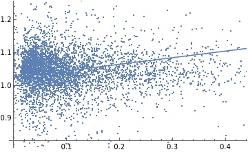
The linear equation above suggests that on average national wealth increases annually by 2.5% due to factors unrelated to trade and at a rate of 4.0% due to trade.
In[]:=
0.201237*Mean[Flatten[tradePct]]
Out[]=
0.0398262
The average annual growth in wealth is 6.5% (≈2.5+4.0%).
In[]:=
Mean[Flatten[growthPct]]
Out[]=
1.06515
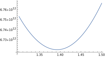
Estimating β (scalar)
Estimating β (scalar)
Finding parameters that minimize the average error (Euclidean distance) between the actual and predicted wealth vectors, for each year from 1996-2020. Assuming β is a scalar and λ = 1.0253. This is a sliding simulation. With this method, β = 1.392.
In[]:=
error[beta_]:=Block[{},μ=30;λ=1.0253;β=beta;Mean[MapThread[EuclideanDistance,{Map[UpdateS,WorldPowerStructureSeries],Rest[WealthSeries]}]]]
In[]:=
results=Map[{#,error[#]}&,Range[1.3,1.5,.001]];ListLinePlot[results]
Out[]=
In[]:=
Take[Sort[Map[Reverse,results]],10]
Out[]=
{{6.72×,1.392},{6.72×,1.393},{6.72×,1.391},{6.72001×,1.394},{6.72002×,1.39},{6.72003×,1.395},{6.72004×,1.389},{6.72006×,1.396},{6.72006×,1.388},{6.72009×,1.397}}
12
10
12
10
12
10
12
10
12
10
12
10
12
10
12
10
12
10
12
10
Law of Motion
Law of Motion
UpdateS
UpdateS
Apply the law of motion to a size vector and components of a tactic matrix. These functions can accept β and λ as either scalars or vectors. Output: size vector.
In[]:=
UpdateS[s_List,Tpos_List?MatrixQ,Tneg_List?MatrixQ,Tzed_List?MatrixQ]:=Ramp[(βTpos-μTneg+λTzed).s]
Apply the law of motion to a size vector and the tactic matrix components from an extended power structure. Output: size vector.
In[]:=
UpdateS[s_List,ps_Association?ExtendedPowerStructureQ]:=UpdateS[s,ps["Tpos"],ps["Tneg"],ps["Tzed"]]
Apply the law of motion to an extended power structure. Output: size vector.
In[]:=
UpdateS[ps_Association?ExtendedPowerStructureQ]:=UpdateS[ps["s"],ps["Tpos"],ps["Tneg"],ps["Tzed"]]
Apply the law of motion to a size vector and the tactic matrix components from an extended power structure, repeatedly to a given depth. Output: size vector.
In[]:=
UpdateS[s_List,ps_Association?ExtendedPowerStructureQ,depth_Integer]:=Fold[UpdateS[#1,#2]&,s,Table[ps,depth]]
SimulateLawOfMotion
SimulateLawOfMotion
Simulate the law of motion over several steps. Output: list of size vectors.
In[]:=
SimulateLawOfMotionS[s_List,ps_Association?ExtendedPowerStructureQ,depth_Integer]:=FoldList[UpdateS[#1,#2]&,s,Table[ps,depth]]
In[]:=
SimulateLawOfMotionS[ps_Association?ExtendedPowerStructureQ,depth_Integer]:=SimulateLawOfMotionS[ps["s"],ps,depth]
Given a list of (extended) power structures, simulate the law of motion over a given time period. The initial size vector comes from the first power structure in the list, and the tactic matrix varies every year based on the other power structures. Output: list of size vectors.
In[]:=
SimulateLawOfMotionDynamicT[pss_]:=FoldList[UpdateS,First[pss]["s"],pss];
Extract simulation data for selected countries (by country ID). Output: list of size vectors.
In[]:=
SimulationSubset[sim_,countryIDs_List]:=Map[#[[countryIDs]]&,sim]
Plot Generation, etc.
Plot Generation, etc.
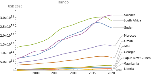
SizeSeriesSubsetPlot
SizeSeriesSubsetPlot
Given a time series of wealth vectors from all countries, extract specified countries and plot them.
In[]:=
SizeSeriesSubsetPlot[sim_,countryIDs_,startYear_,title_]:=ListLinePlot[Map[Transpose[{Range[startYear,startYear+Length[sim]-1],#}]&,Transpose[SimulationSubset[sim,countryIDs]]],PlotLabelsMap[CountryName,countryIDs],AxesLabel{"Year","USD 2020"},PlotLabeltitle,PlotRangeAll]
In[]:=
SizeSeriesSubsetPlot[SmoothedWealthSeries,RandomChoice[Range[193],10],1995,"Rando"]
Out[]=
Comparison Plots
Comparison Plots
Base function that generates the comparison plot.
In[]:=
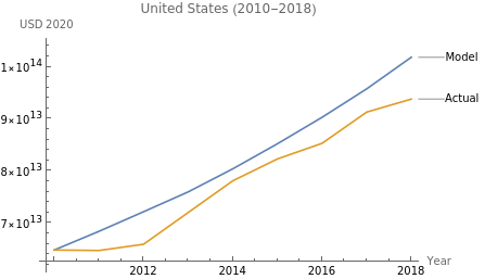
ComparisonPlot[sim_,actual_,countryName_,startYear_,endYear_]:=Block[{},ListLinePlot[Map[Transpose[{Range[startYear,startYear+Length[sim]-1],#}]&,{sim,actual}],PlotLabels{"Model","Actual"},AxesLabel{"Year","USD 2020"},PlotLabelcountryName<>" ("<>ToString[startYear]<>"-"<>ToString[endYear]<>")",PlotRangeAll,TicksRange[startYear,endYear]]]
Compares the actual wealth series to the model, assuming that the initial size vector is iteratively updated based on a tactic matrix that varies every year.
In[]:=
ComparisonPlotDynamicT[countryName_,start_,end_]:=Block[{sim,actual,c=CountryID[countryName]},sim=SimulateLawOfMotionDynamicT[WorldPowerStructure[start+1,end]][[All,c]];actual=Transpose[WealthSeriesInterval[start,end]][[c]];ComparisonPlot[sim,actual,countryName,start,end]]
In[]:=
ComparisonPlotDynamicT["United States",2010,2018]
Out[]=
ReallocateTrade
ReallocateTrade
Reallocate a percentage of a state’s power (trade volume) away from its opponents and towards its allies. The input matrix is assumed to be a trade matrix. Output: trade matrix.
In[]:=
ReallocateTrade[i_Integer,T_,allies_List,opponents_List,pct_]:=Block[{len=Length[T],dT=T,reducedT,diff,add,addT},(*Reducei'stradewithopponentsbypct*)reducedT=ReplacePart[dT,Flatten[Map[{{#,i}dT[[#,i]]*(1.-pct),{i,#}dT[[i,#]]*(1.-pct)}&,opponents]]];(*Totalamountoftradereductionwithopponents*)diff=Total[Map[dT[[i,#]]*pct&,opponents]];(*Reallocationofthattradetoallies*)add=allocationPct[ReplacePart[ConstantArray[0.,len],Map[#dT[[#,i]]&,allies]]]*diff;addT=ReplacePart[ReplaceColumn[ConstantArray[0.,{len,len}],i,add],{iadd}];reducedT+addT]
A version that references global variables, used in a Fold, e.g. Fold[ReallocateTrade,T,allies].
In[]:=
ReallocateTrade[T_,i_]:=ReallocateTrade[i,T,allies,opps,pct]
Normalize the vector of trade allocated to an country’s allies, such that the vector total equals 1.
In[]:=
allocationPct[s_]:=If[Total[s]0.,s,s/Total[s]]
Figures
Figures
Largest Countries by National Wealth (1995-2020)
Largest Countries by National Wealth (1995-2020)
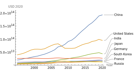
A combined list of the biggest N countries in each year from 1995-2020.
In[]:=
SizeSeriesSubsetPlot[WealthSeries,Map[CountryID,{"China","United States","India","Japan","Germany","South Korea","France","Russia"}],1995,""]
Largest countries by national wealth (1995-2020) |
Basic Comparison Plots
Basic Comparison Plots
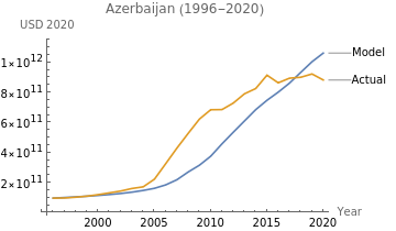
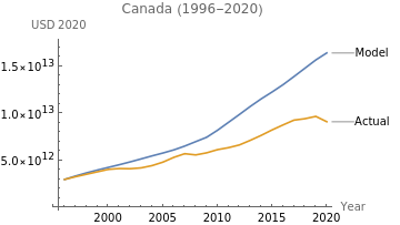
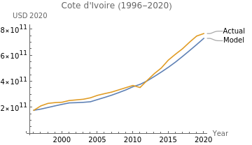
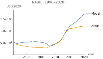
The following are four examples of the model compared to actual national wealth.
In[]:=
ComparisonPlotDynamicT["Azerbaijan",1996,2020]
Out[]=
In[]:=
ComparisonPlotDynamicT["Canada",1996,2020]
Out[]=
In[]:=
ComparisonPlotDynamicT["Cote d'Ivoire",1996,2020]
Out[]=
In[]:=
ComparisonPlotDynamicT["Nauru",1996,2020]
Out[]=
Conflict Comparison Plots
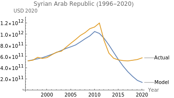
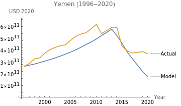
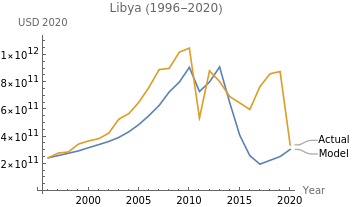
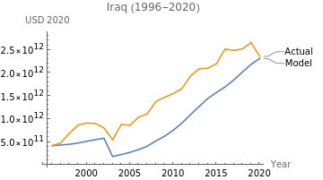
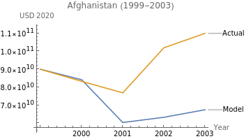
Conflict Comparison Plots
Examples of countries that experienced major conflict.
In[]:=
ComparisonPlotDynamicT["Syrian Arab Republic",1996,2020]
Out[]=
In[]:=
ComparisonPlotDynamicT["Yemen",1996,2020]
Out[]=
In[]:=
ComparisonPlotDynamicT["Libya",1996,2020]
Out[]=
In[]:=
ComparisonPlotDynamicT["Iraq",1996,2020]
Out[]=
In[]:=
ComparisonPlotDynamicT["Afghanistan",1999,2003]
Out[]=
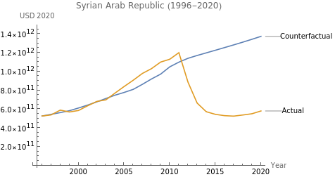
Syria Counterfactual
Syria Counterfactual
Actual wealth series (Syria)
In[]:=
Transpose[WealthSeriesInterval[1996,2020]][[CountryID["Syrian Arab Republic"]]]
Out[]=
{5.26×,5.38×,5.89×,5.69×,5.85×,6.35×,6.81×,6.98×,7.7×,8.4×,9.07×,9.79×,1.03×,1.1×,1.13×,1.2×,8.86×,6.64×,5.72×,5.44×,5.3×,5.25×,5.37×,5.5×,5.8×}
11
10
11
10
11
10
11
10
11
10
11
10
11
10
11
10
11
10
11
10
11
10
11
10
12
10
12
10
12
10
12
10
11
10
11
10
11
10
11
10
11
10
11
10
11
10
11
10
11
10
In[]:=
actual={5.26`*^11,5.38`*^11,5.89`*^11,5.69`*^11,5.85`*^11,6.35`*^11,6.81`*^11,6.98`*^11,7.7`*^11,8.4`*^11,9.07`*^11,9.79`*^11,1.03`*^12,1.1`*^12,1.13`*^12,1.2`*^12,8.86`*^11,6.64`*^11,5.72`*^11,5.44`*^11,5.3`*^11,5.25`*^11,5.37`*^11,5.5`*^11,5.8`*^11};
Counterfactual prediction, assuming no civil war. Note, this requires modifying the Interstate Wars 1995-2020 - DyadYears.csv file.
SimulateLawOfMotionDynamicT[WorldPowerStructure[1997,2020]][[All,CountryID["Syrian Arab Republic"]]]
Out[]=
{5.26×,5.4415×,5.62498×,5.82591×,6.11421×,6.42372×,6.76514×,7.12326×,7.47772×,7.76964×,8.09642×,8.63271×,9.202×,9.71627×,1.04911×,1.09905×,1.13993×,1.17001×,1.1977×,1.22563×,1.25392×,1.28233×,1.31164×,1.342×,1.37343×}
11
10
11
10
11
10
11
10
11
10
11
10
11
10
11
10
11
10
11
10
11
10
11
10
11
10
11
10
12
10
12
10
12
10
12
10
12
10
12
10
12
10
12
10
12
10
12
10
12
10
In[]:=
counterfactual={5.26`*^11,5.4414953032536926`*^11,5.624978498474115`*^11,5.825910383669932`*^11,6.114210548301962`*^11,6.423718289921146`*^11,6.765136598683021`*^11,7.123263673904281`*^11,7.477721225499418`*^11,7.769642542975702`*^11,8.096418080699792`*^11,8.632712592851847`*^11,9.201998424412217`*^11,9.716266289654575`*^11,1.0491138823078627`*^12,1.0990491881822632`*^12,1.139925267033488`*^12,1.1700085899803325`*^12,1.1976989890162507`*^12,1.225628885912731`*^12,1.2539226517444268`*^12,1.282329436046333`*^12,1.3116367170049688`*^12,1.342000723028785`*^12,1.3734263251199226`*^12};
Combining into a plot
In[]:=
startYear=1996;endYear=2020;countryName="Syrian Arab Republic";ListLinePlot[Map[Transpose[{Range[startYear,startYear+Length[actual]-1],#}]&,{counterfactual,actual}],PlotLabels{"Counterfactual","Actual"},AxesLabel{"Year","USD 2020"},PlotLabelcountryName<>" ("<>ToString[startYear]<>"-"<>ToString[endYear]<>")",PlotRangeAll,TicksRange[startYear,endYear]]
Out[]=
Predicted wealth of Syria had it not experienced civil war starting in 2011 |
WW2
WW2
In the following figure, we illustrate the evolution of five major powers (Germany, Japan, Russia, the United Kingdom, and the United States) over the course of World War 2 as we show the reduction in strength of Germany and Japan as the war unfolded. The figure was created with code from another notebook.
Out[]=
Simplified power structure sequence depicting World War 2 |


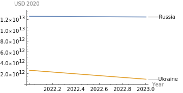
Russo-Ukranian War
Russo-Ukranian War
Wealth as of 2020
In[]:=
WealthVector[2020][[CountryID["Russia"]]]
Out[]=
1.26×
13
10
In[]:=
WealthVector[2020][[CountryID["Ukraine"]]]
Out[]=
2.68×
12
10
Trade volume (2020)
In[]:=
TradeVector[2020][[CountryID["Russia"]]]
Out[]=
5.93516×
11
10
In[]:=
TradeVector[2020][[CountryID["Ukraine"]]]
Out[]=
1.07574×
11
10
Russian military expenditure on Ukraine: assume roughly $300M/day. https://www.themoscowtimes.com/2022/05/18/russian-defense-spending-surges-to-300m-per-day-amid-ukraine-war-a77712
In[]:=
300000000*365
Out[]=
109500000000
Ukraine’s military expenditure on Russia: $8.3 billion from Feb-May. https://www.reuters.com/world/europe/exclusive-war-forces-ukraine-divert-83-bln-military-spending-tax-revenue-drops-2022-05-12/
In[]:=
8300000000*(12/4)
Out[]=
24900000000
Western support for Ukraine (Feb-Aug 2022): Ukraine has received more than $12 billion worth of weapons and financial aid from Western countries since the start of Russia’s invasion, as of May 5. https://www.reuters.com/world/europe/ukraine-gets-over-12-billion-weapons-financial-aid-since-start-russian-invasion-2022-05-05/
In[]:=
12000000000.*(12/7)
Out[]=
2.05714×
10
10
Western trade reductions with Russia (2022): Assume trade volume is reduced by 20%.
In[]:=
TradeVector[2020][[CountryID["Russia"]]]*0.8
Out[]=
4.74813×
11
10
Russia’s wealth after a year of war. Assume that half of military expenditure is applied violence.
In[]:=
rus2023=(λ(WealthVector[2020][[CountryID["Russia"]]]-TradeVector[2020][[CountryID["Russia"]]]*0.8-109500000000))-109500000000-(μ24900000000*0.5)+(βTradeVector[2020][[CountryID["Russia"]]]*0.8)
Out[]=
1.2494×
13
10
Ukraine’s wealth after a year of war. Assuming Ukraine’s trade volume drops by 50%. Assume that half of military expenditure is applied violence.
In[]:=
ukr2023=(λ(WealthVector[2020][[CountryID["Ukraine"]]]-TradeVector[2020][[CountryID["Ukraine"]]]-24900000000))-24900000000-(μ109500000000*0.5)+(βTradeVector[2020][[CountryID["Ukraine"]]]*0.5)+2.057142857142857`*^10
Out[]=
1.03926×
12
10
In[]:=
ukr2023/WealthVector[2020][[CountryID["Ukraine"]]]
Out[]=
0.387782
Plot of the results
In[]:=
startYear=2022;endYear=2023;ListLinePlot[Map[Transpose[{Range[startYear,startYear+Length[rus]-1],#}]&,{{WealthVector[2020][[CountryID["Russia"]]],rus2023},{WealthVector[2020][[CountryID["Ukraine"]]],ukr2023}}],PlotLabels{"Russia","Ukraine"},AxesLabel{"Year","USD 2020"},PlotRangeAll,TicksRange[startYear,endYear]]
Out[]=
World Power Structure Matrix
World Power Structure Matrix
Produces a matrix of the WPS for a given year.
In[]:=
WPSMatrix[year_]:=(βTpos[year]-μTneg[year]+λTzed[year])
In[]:=
MatrixPlot[WPSMatrix[2020],FrameFalse]
Out[]=
World power structure: interstate relationships in 2020 |
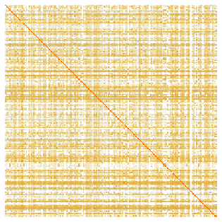
Each column in this 193x193 matrix represents a state’s “foreign policy” towards every other state, with brighter colors denoting more activity. Negative values, indicating destruction, are in blue, but there are only a few dozen of them and they are so faint as to be invisible, illustrating that the vast majority of state interaction in the contemporary international system is constructive. The orange diagonal is the power that each state does not set in motion but retains as a stock.
Number of negative values in the matrix above:
In[]:=
Count[Sign[Flatten[WPSMatrix[2020]]],-1]
Out[]=
25
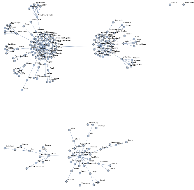
International Trade Network (ITN)
International Trade Network (ITN)
Display a graph of the international trade network for a given year. This shows each country’s primary trading partner.
In[]:=
ITNGraph[year_]:=Block[{T},T=Transpose[Map[OneHotEncodeMax,Transpose[TradeMatrix[year]]]];T=Sign[T+Transpose[T]];AdjacencyGraph[T,VertexLabelsMapIndexed[First[#2]CountryName[#1]&,Range[193]]]]
International Trade Network, 2020 (with Chinese, American, and German clusters).
In[]:=
ITNGraph[2020]
World power structure: primary trading partner relationships, 2020. |
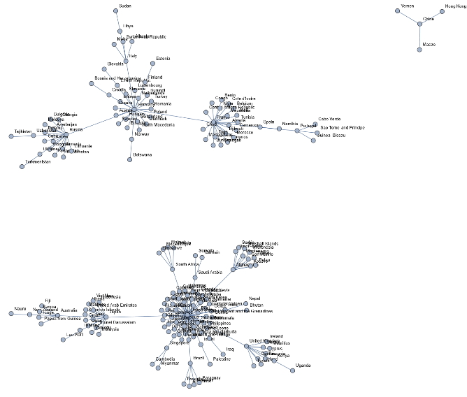
International Trade Network, 1996 (with American, European, and Chinese clusters).
In[]:=
ITNGraph[1996]
Out[]=
Current trajectory: US and China
Current trajectory: US and China
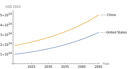
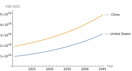
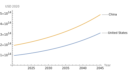
Current growth trajectories of the U.S. and China. When we run a naive simulation of the law of motion based on the 2020 world power structure, the model predicts an increasingly unipolar system dominated by China.
In[]:=
sim=SimulateLawOfMotionS[WorldPowerStructure[2020],25];SizeSeriesSubsetPlot[sim,Map[CountryID,{"United States","China"}],2020,""]
Out[]=
Projected growth in power, China and the U.S. |
Hypothetical ITN: Representative scenario from Swing States
Hypothetical ITN: Representative scenario from Swing States
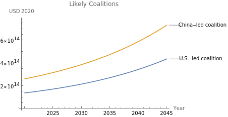
Predicted growth of the U.S.- and China-led coalitions, given a likely scenario. Reference is to: Poulshock, Michael. Swing States in Great Power Competition (2022). Available at: https://papers.ssrn.com/sol3/papers.cfm?abstract_id=4124778.
In[]:=
us=Map[CountryID,{"Afghanistan","Algeria","Antigua and Barbuda","Aruba","Bahamas","Bahrain","Barbados","Bermuda","Canada","Costa Rica","Cyprus","Dominica","Dominican Republic","Ecuador","Gabon","Guatemala","Haiti","Iceland","Maldives","Mexico","Micronesia","Panama","Saint Kitts and Nevis","Saint Lucia","Saint Vincent and the Grenadines","Samoa","Seychelles","Singapore","Taiwan","Trinidad and Tobago","Tuvalu","United States"}];china=Map[CountryID,{"Albania","Angola","Armenia","Australia","Austria","Azerbaijan","Belgium","Bosnia and Herzegovina","Brunei Darussalam","Burkina Faso","Burundi","Cambodia","Cameroon","Central African Republic","China","Colombia","Comoros","Congo","Croatia","Czech Republic","DR Congo","Equatorial Guinea","Georgia","Guinea","Guinea-Bissau","Hong Kong","Hungary","Indonesia","Iraq","Ireland","Jamaica","Kazakhstan","Kiribati","Kosovo","Kyrgyzstan","Lao PDR","Lesotho","Liberia","Mali","Mauritius","Moldova","Myanmar","Namibia","Nauru","Nepal","Netherlands","Niger","North Macedonia","Palestine","Romania","Rwanda","Serbia","Slovakia","Solomon Islands","South Africa","Sri Lanka","Tanzania","Turkmenistan","Uganda","Uruguay","Uzbekistan","Yemen","Zambia","Zimbabwe"}];T=TradeMatrix[2020];pct=.1;allies=us;opps=china;newT=Fold[ReallocateTrade,T,allies];allies=china;opps=us;newT=Fold[ReallocateTrade,newT,allies];
Growth of China and U.S. in simulation
In[]:=
ps=PowerStructure[WealthVector[2020],NormalizeT[NormalizationVector[2020],newT],Tneg[2020]];sim=SimulateLawOfMotionS[ps,25];SizeSeriesSubsetPlot[sim,Map[CountryID,{"United States","China"}],2020,""]
Out[]=
Total wealth of each coalition
In[]:=
blue=Total[Transpose[sim][[us]]];red=Total[Transpose[sim][[china]]];ListLinePlot[Map[Transpose[{Range[2020,2020+Length[sim]-1],#}]&,{blue,red}],PlotLabels{"U.S.-led coalition","China-led coalition"},AxesLabel{"Year","USD 2020"},PlotRangeAll,PlotLabel"Likely Coalitions"]
Out[]=
Projected power of coalitions led by the U.S. and China: likely |
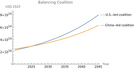
Hypothetical ITN: Balancing Coalition from Swing States
Hypothetical ITN: Balancing Coalition from Swing States
Predicted growth of the U.S.- and China-led coalitions, given a balancing scenario. Reference is to: Poulshock, Michael. Swing States in Great Power Competition (2022). Available at: https://papers.ssrn.com/sol3/papers.cfm?abstract_id=4124778.
In[]:=
us=Map[CountryID,{"United States","Canada","Japan","Germany","South Korea","France","Taiwan","United Kingdom","Spain","Australia"}];china=Map[CountryID,{"China","Russia","Iran","Pakistan","Indonesia","United Arab Emirates","Nigeria"}];T=TradeMatrix[2020];pct=.1;allies=us;opps=china;newT=Fold[ReallocateTrade,T,allies];allies=china;opps=us;newT=Fold[ReallocateTrade,newT,allies];
Growth of China and U.S. in simulation
In[]:=
ps=PowerStructure[WealthVector[2020],NormalizeT[NormalizationVector[2020],newT],Tneg[2020]];sim=SimulateLawOfMotionS[ps,25];SizeSeriesSubsetPlot[sim,Map[CountryID,{"United States","China"}],2020,""]
Out[]=
Total wealth of each coalition
In[]:=
blue=Total[Transpose[sim][[us]]];red=Total[Transpose[sim][[china]]];ListLinePlot[Map[Transpose[{Range[2020,2020+Length[sim]-1],#}]&,{blue,red}],PlotLabels{"U.S.-led coalition","China-led coalition"},AxesLabel{"Year","USD 2020"},PlotRangeAll,PlotLabel"Balancing Coalition"]
Out[]=
Projected power of coalitions led by the U.S. and China: U.S.-ledbalancing coalition |