CITE THIS NOTEBOOK: Analytic continuation done right with ReImPlot in a row by Shenghui Yang. Wolfram Community DEC 26 2022.
Forget about the fancy Riemann surface 3D graphics you saw online. The 3D are quite difficult to understand because the intersection you see in the surface are just hallucination from the projection. Instead, use the following ReImPlots + GraphicsRow to understand what is behind branch cut. Also you should treat RS as mapping between gamepads stick movement (z) and the motion of the character on the monitor f(z). In this way you can imagine 4D space mapping intuitively.The article also serves as a nice companion to understand YouYuber “qncubed3”’s “Complex Analysis: Fancy Branch Cuts”
Simple case for radicals
Simple case for radicals
The can be analytical continue itself automatically beyond one round:
z
In[]:=
ReImPlot[Exp[*θ/2],{θ,-π,π}]
Out[]=
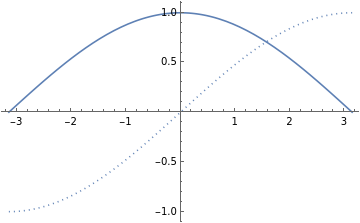
When you turn twice along the circle centered at , you comes back. Nothing more to be done in this case.
z
z=0
In[]:=
g1=ReImPlot[Exp[*θ/2],{θ,-π,3π},PlotRange->{-1.2,1.2},PlotRangePadding->0]
Out[]=
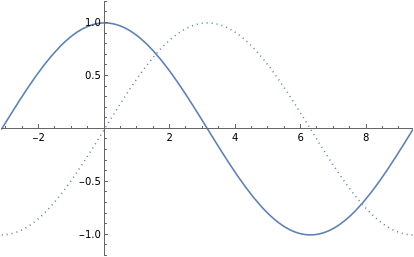
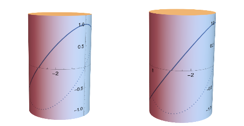
We can safely roll the graph on to a cylinder and the curves two ends meet nicely respectively:
In[]:=
textCyl=Graphics3D[{Texture[g1],EdgeForm[],cyl[{{0,0,0},{0,0,2Pi}},2,19]},Boxed->False];
In[]:=
{textCyl,textCyl}//Row
Out[]=
Or simply combine the external such that =θ+2π. Since θ is from -π to π, is from π to 3π:
θ
2
θ
2
In[]:=
Labeled[GraphicsRow[{ReImPlot[Exp[*θ/2],{θ,-π,π},Ticks->{{-π,-π/2,0,π/2,π},{-1,1}}],ReImPlot[Exp[*θ/2],{θ,π,3π},Ticks->{{π,3π/2,2π,3π},{-1,1}}]}],"Analytical coninuation of ",Top]//Framed
z
Out[]=
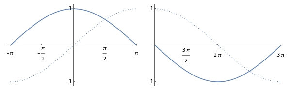
Notice that it is the key to keep in the expression. It indicates that we should add an angle shift
π
More advanced examples
More advanced examples
We have two branch cuts -1 and we go around on circle :
2
z
|z|=2
In[]:=
ComplexPlotz,{z,1},,ComplexPlot//GraphicsRow
(z)^2-1
,{z,-2},Out[]=
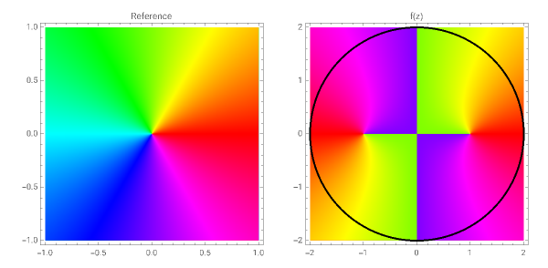
Check its Riemann surface with ReImPlot:
In[]:=
ReImPlot
(2*Exp[*θ])^2-1
,{θ,-π,π},PlotLegends->"ReIm"Out[]=
This about the whole expression as . Therefore we need to think about etc. We multiply at the out most expression to indicate that it is from and :
(1/2(Exp[*θ])^2-1)
u
Arg(u)=θ,θ+/-2π,θ+/-3π
(*π)
Arg(u)/2=θ/2
(θ+2π)/2=θ/2+π
In[]:=
ReImPlotExp[*π]
(2*Exp[*θ])^2-1
,{θ,-π,π}Out[]=
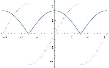
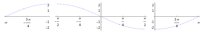
The analytic continuation, from (-π,-π/2) to (-π/2,π/2) and then to (π/2,π), is again checked by put three graphics in a row. Because the winding number is two from the complex plot above, we can safely omit half of the plot because that’s just a flip of the diagram below:
In[]:=
LabeledReImPlot,ReImPlotExp[*π],ReImPlot//GraphicsRow,"Analytic Continuation for Re(f(z))",Top//Framed
(2Exp[*θ])^2-1
,{θ,-π,-π/2},(2Exp[*θ])^2-1
,{θ,-π/2,π/2},(2Exp[*θ])^2-1
,{θ,π/2,π},Out[]=
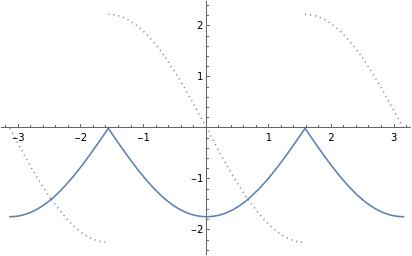
In[]:=
LabeledReImPlotSqrt[(2Exp[I*θ])^2-1],{θ,-π,-π/2},,ReImPlotExp[I*π]Sqrt[(2Exp[I*θ])^2-1],{θ,-π/2,π/2},,ReImPlot//GraphicsRow,"Analytic Continuation for Im(f(z))",Top//Framed
Out[]=
This separated graphs also shows in general Riemann surface does not intersects like those shown in 3D projection.
Branch cut with log function
Branch cut with log function
Let’s look at the function :
f(x)
Out[]//TraditionalForm=
log(+1)
4
x
2
x
which has a nice integral from to :
-∞
+∞
In[]:=
Integrate[Log[x^4+1]/(x^2+1),{x,-∞,∞}]
Out[]=
πLog[6+4
2
]I will skip how to use the branch cut to find the integral because it is well demonstrated in this YouTube lecture by “qncubed3”. We only study the associated property of the branch cut.
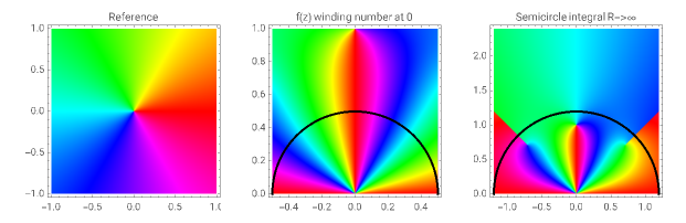
Check its topology on the upper half complex plane (number of poles, zeros and branch cuts)
In[]:=
ComplexPlotz,{z,1},,ComplexPlotLog[z^4+1](z^2+1),{z,-1/2,1/2+},,ComplexPlotLog[z^4+1](z^2+1),{z,-2.4/2,2.4/2+2.4},//GraphicsRow
Out[]=
For small region around origin, it is entire. The topological space is a cylinder/Complex plane quotient one-d lattice because you can wrap the following diagram on cylinder by joining the Re/Im curve at and , just like at point zero (the function repeat twice )
-π
π
ReImPlot[Evaluate[Log[x^4+1]/(x^2+1)/.x->(0.9Exp[*θ])],{θ,-π,π}]
Out[]=
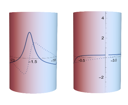
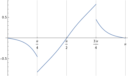
Wrap half of the graph above on to a cylinder. Still no jump when we join the two ends:
In[]:=
Withg2=,Graphics3D[{Texture[g2],EdgeForm[],cyl[{{0,0,0},{0,0,2Pi}},2,19]},Boxed->False]
Out[]=
For slightly larger semicircle, it will go through two branch cuts at π/4 and 3π/4:
In[]:=
ComplexPlot[Log[z^4+1]/(z^2+1),{z,1.5},PlotLegendsAutomatic,PlotPoints->50,RasterSize->600,Epilog->{Circle[{0,0},1.3,{0,π}],Arrow[{{-1.3,0},{1.3,0}}]}]
Out[]=
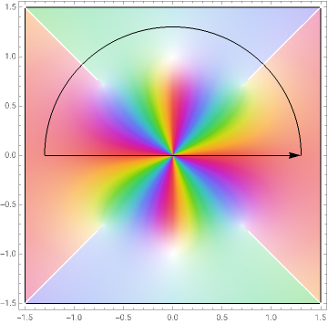
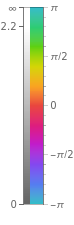
This means we will see the the jump in imaginary part because the branch cut effects the log function:
In[]:=
Plot[Evaluate[Im[Log[x^4+1]/(x^2+1)/.x->(2Exp[*θ])]],{θ,0,π},PlotPoints->50,Ticks->{{0,π/4,π/2,3π/4,π},Automatic},GridLines->{{0,π/4,π/2,3π/4,π},None}]
Out[]=
We need analytic continuation to understand how the branch cut affects the choice of integration path. You probably have seen the spiral for the imaginary part of . The imaginary part of the function goes with as can be extended beyond principle range . You can take the spiral -elevator upward and downward, whichever way you like.
Log(z)
θ
ImLog()=θ
θ
{-π,π}
θ
In[]:=
Riemann surface of log z
Lets check how we can use analytical continuation to extend beyond the interval {0,π/4}:
In[]:=
ReImPlot[Evaluate[Log[x^4+1]/(x^2+1)/.x->(2Exp[*θ])],{θ,0,π/4},PlotPoints->50]
Out[]=
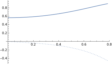
Compute the value of imaginary part at branch cut by approaching from below
In[]:=
discon=Im[Log[x^4+1]/(x^2+1)/.x->(2Exp[*π/4.])]
Out[]=
-0.452389
Notice that the branch cut spiral for Im is from Log alone. So we need to compensate the imagine part discontinuity on the Log part! This is totally different from adding directly to .
2π
Im(f(z))
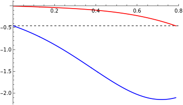
Join discontinuity at if we plot them in them in the same graph the ends can be joined with a horizontal line:
θ=π/4
In[]:=
Plot[Evaluate@{Style[Im[Log[x^4+1]/(x^2+1)/.x->(2Exp[*θ])],Red],Style[Im[(Log[x^4+1]+2π*I)/(x^2+1)/.x->(2Exp[*(θ+π/4)])],Blue],},{θ,0,π/4},PlotPoints->50,GridLines->{None,{discon}},GridLinesStyle->Directive[{Thickness[0.006],Dashed,Gray}]]
Out[]=
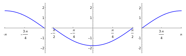
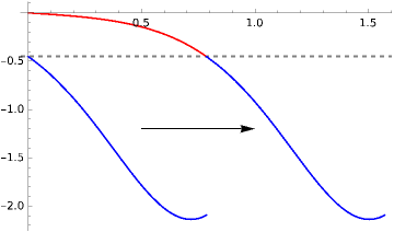
If we translate the lower part along the dashed line, it should match perfectly with the upper half. We simplify the function a little bit here. Also use a smaller range for the second part of the piecewise function for the convenience visualization:
In[]:=
continuation[θ_]=PiecewiseIm,0<θ<π4,Im,π4<θ<π2,Indeterminate
Log[1+16]
4θ
1+4
2θ
2π+Log[1+16]
4θ
1+4
2θ
Out[]=
|
The analytic continuation is now perfectly done if we do not jump and go to the “lower” level.
In[]:=
Plot[{continuation[θ],continuation[θ+π/4]},{θ,0,π/2},GridLines{None,{discon}},GridLinesStyleDirective[{Thickness[0.006`],Dashed,Gray}],ColorFunctionFunction[{x,y},If[y>discon,Red,Blue]],ColorFunctionScalingFalse,Epilog->Arrow[{{0.5,-1.2},{1.0,-1.2}}]]
Out[]=
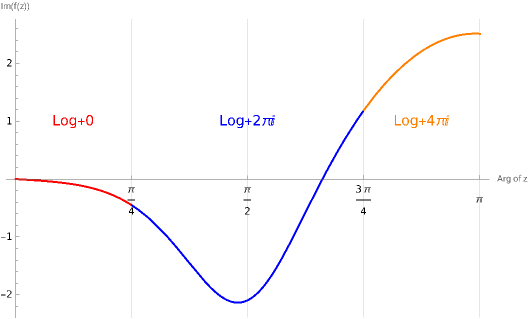
The actual path for lower level if we complete the semi-circle and across two branch cut is
pw=PiecewiseIm,0<θ<π4,Im,π4<θ<3π4,Im,3π4<θ<π,Indeterminate
Log[1+16]
4θ
1+4
2θ
2π+Log[1+16]
4θ
1+4
2θ
4π+Log[1+16]
4θ
1+4
2θ
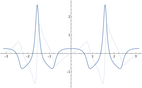
All section are colored and the analytic continuation with corresponding supplementary ’s are labeled with same color:
2π
In[]:=
Plotpw,{θ,0,π},
Out[]=
The analysis can be easily carried to other part of the complex surface using the same technique
Summary
Summary
The idea of this article is to give a accessible approach to understand Riemann surface for those function with branch cuts. You really don’t need the 3D surface to understand the mechanism. ReImPlot gives a very straightforward way to show you how to stitch different part of Riemann surface altogether by shifting and add.
This work is inspired by, in addition to the YouTube video mentioned, a great lecture about this topic long time ago. I regarded this as forever shining gem in the history of pedagogy of advanced mathematics.
This work is inspired by, in addition to the YouTube video mentioned, a great lecture about this topic long time ago. I regarded this as forever shining gem in the history of pedagogy of advanced mathematics.
Out[]=
Utility function
Utility function