Kretschmann scalar for hypergraphs
by Ariadna Uxue Palomino Ylla
Pontifical Catholic University of Peru
by Ariadna Uxue Palomino Ylla
Pontifical Catholic University of Peru
The scope of this project is to look for a discrete analogue of the Kretschmann scalar that can be applied to hypergraphs. The particular approach we take is based on the geometric interpretation of the Weyl curvature on a geodesic ball. We propose that the discrepancy between the number of geodesic paths of a point to different points on its boundary measures the Weyl tensor for this point. In this sense, as the Kretschmann scalar (in an empty space) is just a generalization of the trace of the Weyl tensor, we compute a measure of deviation for all directions to represent this trace. We use hypergraphs produced by a random sprinkling of points into a 3-dimensional Riemannian manifold with extrinsic curvature to calculate the Kretschmann scalar and measure the correlations between this and the estimated we proposed. We do not find a clear correlation in small sprinkled hypergraphs, but the results for 100 to 500 hypergraph vertices seem to indicate a non-stable convergence.
Introduction
Introduction
To better understand the relation of general relativity to hypergraphs in the context of the Wolfram Model, the comprehension of geometric properties is important. In particular, the Kretschmann scalar represents the curvature of the spacetime in the vicinity and within black holes as a function of the radial distance to its center. This project aims to find a discrete analogue of this scalar to have a better understanding of the curvature and its appearance in hypergraphs. The Riemann tensor describes the tidal force on a body moving along a geodesic. The Ricci decomposition is a procedure in differential geometry that essentially describes how the Riemann curvature tensor can be decomposed into a sum of and , which represent the trace part, and , the traceless part. The trace part is related to the Ricci curvature and it contains information on the volume changes, while the traceless part is the Weyl tensor. This tensor does not contain any information on the volume changes but only on the shape change produced by the tidal force. In a vacuum solution, the invariants of the Weyl tensor and of the Riemann tensor (the Kretschmann scalar) coincide. By estimating a discrete analogue that conveys the information of the Weyl tensor, we can find a quantity related to the Kretschmann scalar. We estimate the shape change of an hypergraph by a geometric definition supported on the discrepancy between geodesic paths on geodesic ball boundaries. In order to refine this geometric intuition a power series expansion for the tidal deformation of a geodesic ball in terms of the Weyl tensor is needed.
S
ρσμν
E
ρσμν
W
ρσμν
Some key concepts
Some key concepts
In general relativity (GR), the spacetime is described by a smooth orientable manifold ℳ with a Lorentzian metric ℊ and an associated covariant derivative operator for the metric connection ∇. This manifold is locally similar to the well-known flat Minkowski spacetime from special relativity. An interesting feature in GR is that massive bodies produce changes in the curvature of spacetime. Our Sun, with a mass of approximately , only gives rise to a slight change in curvature. However, other objects as black holes, with masses ranging from 3 to 10 times the solar mass, produce substantial changes in the curvature of the space-time grid. This, in turn, introduces a nontrivial topology on the spacetime [4].
1.99kg
30
10
Plotting a Flamm’s paraboloid to qualitatively compare the spatial curvature produced by a black hole (in the center of the M87 galaxy) and our Sun in the Schwarzschild solution
In[]:=
ParametricPlot3DEvaluaterCos[θ],rSin[θ],(4(r/rs-1))/.{{rs->1.9*},{rs->2.95*}},{θ,0,2π},{r,0,},PlotRangeAll,PlotLegends{"Black Hole","Sun"},PlotStyle{Black,RGBColor[0.96,0.31,0.16]},AxesLabel->{"x [m]","y [m]","z [m]"},LabelStyle->Directive[Bold,10],ImageSizeLarge,ViewPoint{0,-2,0.5}
2
rs
13
10
3
10
14.3
10
Out[]=

A manifold is regular if the metric is , in this sense a manifold that presents a singularity is a non-regular manifold. To check the regularity of space-time the Kretschmann scalar is often used. It is especially useful for vacuum solutions of the Einstein equations, as in the Schwarzschild spacetime, where the Ricci curvature vanishes even when this manifold is not flat [2].
The Kretschmann scalar is a curvature invariant obtained from the Riemann curvature tensor. In general, curvature scalars come from tensors that represent curvature, such as the Ricci or Riemann tensors. Most of the time we think of the curvature in terms of the Gaussian curvature, which is also obtained from the Riemann tensor by contraction of the second and fourth indices. However, this particular scalar does not allow us to measure curvature in vacuum solutions, and therefore prevents us from studying black holes.
2
C
K
The Kretschmann scalar is a curvature invariant obtained from the Riemann curvature tensor. In general, curvature scalars come from tensors that represent curvature, such as the Ricci or Riemann tensors. Most of the time we think of the curvature in terms of the Gaussian curvature
R
The derivation of those curvature scalars is simple to carry out. For an specified metric ℊ, we can define a normal coordinate system at a point m ϵ ℳ, by means of the metric connection ∇. The Riemann tensor obtained from this connection conveys all the information on the geometric curvature. To calculate the Riemann tensor we first calculate the Christoffel symbols of the second kind or connection coefficients, an array of numbers which describes the metric connection [1].
()
η
x
η=0,..,n
σ
Γ
μν
1
2
δσ
ℊ
∂
ℊ
νδ
∂
μ
x
∂
ℊ
μδ
∂
ν
x
∂
ℊ
νμ
∂
δ
x
With this connection the Riemann tensor can be calculated as:
ρ
R
σμν
∂
∂
μ
x
ρ
Γ
σν
∂
∂
ν
x
ρ
Γ
σμ
δ
Γ
σν
ρ
Γ
δμ
δ
Γ
σμ
ρ
Γ
δν
To calculate the Kretschmann scalar and the Ricci scalar we have to make some contractions on the Riemann tensor = and = (the Ricci tensor):
K
R
R
κσμν
ℊ
κρ
ρ
R
σμν
R
αβ
δ
R
αδβ
K=R=
αβγδ
R
R
αβγδ
αδ
ℊ
R
δα
The Ricci decomposition is a way of decomposing the Riemann curvature tensor into a sum of tensors which allow us to separate the trace part (+) from the traceless part (the Weyl tensor).
E
ρσμν
S
ρσμν
W
ρσμν
R
ρσμν
E
ρσμν
S
ρσμν
W
ρσμν
An important relation derived from this decomposition is:
W
ρσμν
ρσμν
W
4
R
ij
ij
R
n-2
2
2
R
(n-1)(n-2)
where n = 4, the number of dimensions of the manifold.
Discrepancy between geodesic paths on geodesic ball boundaries
Discrepancy between geodesic paths on geodesic ball boundaries
Geodesics are length-minimizing curves on a manifold. On a hypergraph, a geodesic path is defined by the minimum number of edges that connect two vertexes. In this context, a geodesic ball is defined by using a geodesic as a radius on a graph.
Constructing a grid graph of 10 x 10 vertexes and a hypergraph with the transformation rule {{1, 2, 1}, {1, 3, 4}} {{4, 5, 4}, {5, 4, 3}, {1, 2, 5}}:
In[]:=
graph0=GridGraph[{10,10}];rule1={{{1,2,1},{1,3,4}}{{4,5,4},{5,4,3},{1,2,5}}};graph1=UndirectedGraph@ResourceFunction["HypergraphToGraph"][ResourceFunction["WolframModel"][rule1,Automatic,1000,"FinalState"]];
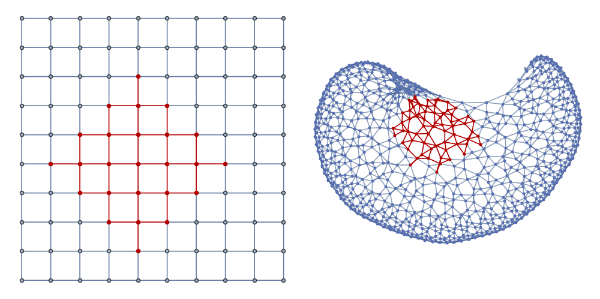
Picking a point in the middle for both graphs and plotting a geodesic ball around them with radius 4:
In[]:=
medio1=GraphCenter[graph1]//First;medio0=GraphCenter[graph0]//First;GraphicsRow[{sphere[graph0,3,medio0],sphere[graph1,4,medio1]},ImageSize600]
Out[]=
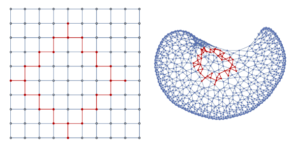
We define a connected boundary by taking the complement of a radius-r ball a radius-(r-1) ball. The boundary has to be connected to define a unique volume by enclosing a region.
In[]:=
GraphicsRow[HighlightGraph[#[[1]],Subgraph[#[[1]],boundary[#[[1]],4,#[[2]]]]]&/@{{graph0,medio0},{graph1,medio1}},ImageSize600]
Out[]=
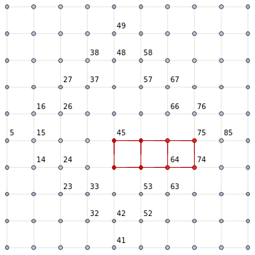
The union of all the geodesic paths defines a volume bound by all the geodesics of some length from the center to a boundary point.
The points on a radius-4 boundary of the 45 vertex are:
In[]:=
b0=boundary[graph0,4,medio0]
Out[]=
{5,15,14,24,16,26,23,33,27,37,32,42,38,48,41,52,49,58,53,63,57,67,64,74,66,76,75,85}
Plots of the volumes defined by the bounded region by all the geodesics between a point in the center and each point of the boundary:
In[]:=
ListAnimate[Table[HighlightGraph[Graph[graph0,EdgeStyleDirective[Gray,Opacity[0.2]],VertexLabelsJoin[Inner[Rule,b0,b0,List],{medio0->medio0}]],Subgraph[graph0,FindAllShortestPaths[graph0,medio0,a]]],{a,b0}],AnimationRunningFalse]
Out[]=
We took the discrepancy of the number of geodesic paths of all the points on the boundary to the center. After studying our preliminary results, we decided to calculate this discrepancy by a “cubic mean deviation” , where is the number of geodesic paths from the center to a point i in a boundary that have a m points. is the mean of all the number of paths. This deviation was chosen because, unlike the mean absolute deviation, it conserves sign information.
cmd=
m
∑
i=1
3
(-)
x
i
x
x
i
x
Further explanation on the discretization process of geometric objects is extensively explained in [3].
Geometric intuition approximation to the Weyl tensor and the Kretschmann scalar
Geometric intuition approximation to the Weyl tensor and the Kretschmann scalar
As the Weyl tensor is related to the shape distortion, let us consider a geodesic ball being stretched by its sides on an axis. If we look at the total number of paths from one of the points in the center to a point on a geodesic ball’s boundary centered on it, that number is going to be larger for the paths that connect the center point to the furthest out points on the boundary and smaller for the paths that go to the closest points.
So by looking at the difference in the number of paths between a particular direction and the perpendicular direction we are essentially estimating an analog to the Weyl curvature tensor. In this case, we are not picking a particular direction but instead, we took an average discrepancy for all directions which conveys a generalized trace (a tensor contraction) of our estimated analog. As the tensor contraction of the Weyl curvature tensor in the vacuum is the Kretschmann scalar, we have to take the average discrepancy of the number of paths across the surface. However, the number of paths between two points can be a huge number, and hence difficult to compute. To solve this difficulty, we took the number of geodesics instead as a representative measure.
A brief comparison
A brief comparison
We produced some hypergraphs by sprinkling points within a 3 dimensional Riemannian manifold with a hyperboloidal extrinsic curvature. By producing these hypergraphs we obtain vertices with coordinates (obtained from the Riemannian metric) that allow us to calculate the Kretschmann scalar with its formal definition.
For each manifold, we produced a group of hypergraphs. Each group is conformed by 5 hypergraphs which go from 100 to 500 vertex. We calculated the Kretschmann scalar for all vertex and also we estimated our candidate to the Kretschmann scalar for fixed radii of 3 and 6. We did this to obtain a qualitative comparison and to do a convergence analysis between our estimated candidate and the known scalar value.
Hyperboloid
Hyperboloid
Assume a 2D submanifold embedded in a 3D Riemannian manifold. By choosing a parametrization as:
X(μ,ν)=(Cosh[ν]Cos[μ],Cosh[ν]Sin[μ],Sinh[ν]),
we obtain a Kretschmann scalar of the form:
In[]:=
KHyperboloid=4;
4
Sech[ν]
In a hyperboloidal manifold the Kretschmann scalar depends only on the second coordinate ν.
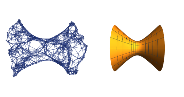
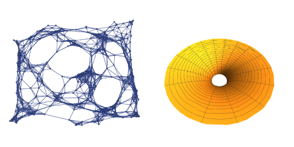
Calculation and plotting of a sprinkling hyperboloid hypergraph of 510 vertex and a paraboloid surface:
manifold1=ECMTG[x^2+y^2-z^21,{x,y,z},{{-3,3},{-3,3},{-3,3}},0.8,510]["PureSpatialGraph"];paraboloid=ParametricPlot3D[{Sinh[ν],Cosh[ν]Cos[μ],Cosh[ν]Sin[μ]},{μ,0,2π},{ν,-ArcSinh[3],ArcSinh[3]},ViewPointFront,BoxedFalse,Axes->False];
GraphicsRow[{manifold1,paraboloid}]
Out[]=
Constructing 5 hypergraphs with 100 to 500 vertices:
max=500;data=ParallelTable[ECMTG[x^2+y^2-z^21,{x,y,z},{{-3,3},{-3,3},{-3,3}},2.5-n/max+0.1*KroneckerDelta[n,10],n]["PureSpatialGraph"],{n,100,max,1}];
Obtaining the graph without coordinates and the lists of vertices (both with coordinates and without them):
graphin2=IndexGraph@data;pointsi2=VertexList@graphin2;coordpointsi2=VertexList@data;
Calculating Kretschmann “real” values:
In[]:=
rvali2=Solve[Sinh[ν]#,{ν}]&/@coordpointsi2〚;;,3〛;
In[]:=
kri2=Flatten[(KHyperboloid/.rvali2),{2,1}];
Let us fix a radio of 3, to only vary the density of vertices.
Cubic Mean Deviation estimator:
Cubic Mean Deviation estimator:
CMD3=ParallelMap[Apply[MeanDeviationfor3,#]/3&,ParallelTable[Thread[{3,Sequence@@a}],{a,Transpose[{graphin2,pointsi2}]}],{2}];CMDi3200=CMD3[[2]]
Let us fix radio of 6, to only vary the density of vertices.
Cubic Mean Deviation estimator:
Cubic Mean Deviation estimator:
CMD6=ParallelMap[Apply[MeanDeviationfor3,#]/6&,ParallelTable[Thread[{6,Sequence@@a}],{a,Transpose[{graphin2,pointsi2}]}],{2}];CMDi6200=CMD6[[2]]
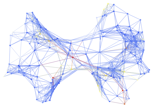
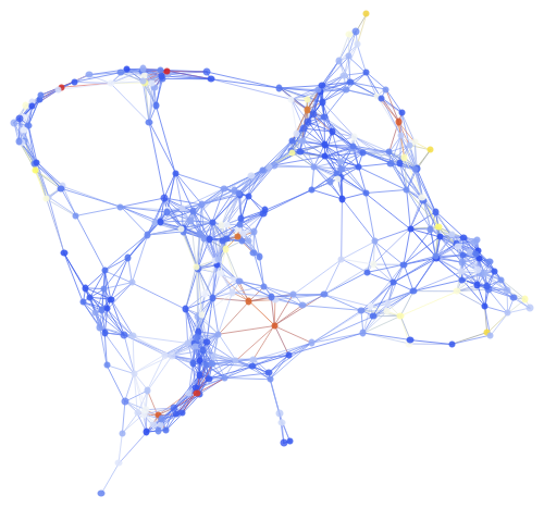
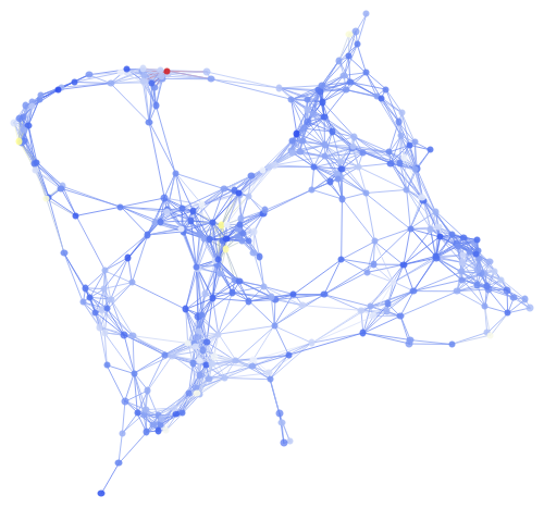
Kretschmann analogue estimated with Cubic Mean Deviation on the left and the former Kretschmann scalar calculated with the coordinates of the vertices on the right for a 200 vertex hypergraph (r = 3):
In[]:=
Row[ColorGraph[graphin2,Transpose[{pointsi2,#}],500,1]&/@{CMDi3200,kri2}]
Out[]=
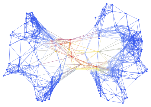
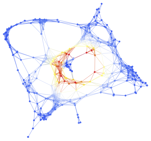
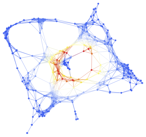
Kretschmann analogue estimated with Cubic Mean Deviation on the left and the former Kretschmann scalar calculated with the coordinates of the vertices on the right for a 200 vertex hypergraph (r = 6):
In[]:=
Row[ColorGraphb[graphin2,Transpose[{pointsi2,#}],500,1]&/@{CMDi6200,kri2}]
Out[]=
Calculating the correlation coefficient and the correlation test for radii 3 and 6:
ρ
0
In[]:=
cρ3i2=Correlation[CMDi3200,kri2]
Out[]=
0.0734091
In[]:=
CP3i2=CorrelationTest[Transpose[{CMDi3200,kri2}],cρ3i2]
Out[]=
0.0186083
cρ6i2=Correlation[CMDi6200,kri2]
Out[]=
0.163949
In[]:=
CP6i2=CorrelationTest[Transpose[{CMDi6200,kri2}],cρ6i2]
Out[]=
0.204728
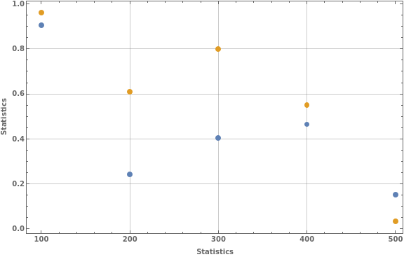
Taking all the correlation test results for the 5 graphs:
In[]:=
ListPlot[{{CP3i1,CP3i2,CP3i3,CP3i4,CP3i5},{CP6i1,CP6i2,CP6i3,CP6i4,CP6i5}},DataRange{100,500},PlotLegends{"r=3","r=6"},FrameLabel{"Number of points","Statistics"},GridLinesAutomatic,FrameTrue,ImageSizeLarge,LabelStyle->Directive[Bold,10]]
Out[]=
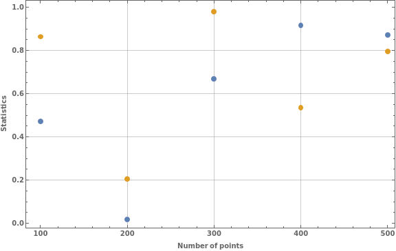
We notice slight indications of convergence, but hypergraphs with more points are needed.
Flamm’s paraboloid
Flamm’s paraboloid
By choosing a parametrization as:
X(r,θ)=rCos[θ],rSin[θ],2
r-1
,we obtain a Kretschmann scalar of the form:
In[]:=
KHFlamm=;
4
2
(-1+r)
6
r
In this manifold the Kretschmann scalar depends only on the second coordinate r.
Calculation and plotting of a sprinkling Flamm’s paraboloid hypergraph of 400 vertices and a surface:
manifold2=ECMTG2Re-z==0,{x,y,z},{{-5,5},{-5,5},{-20,10}},1.3,400["PureSpatialGraph"];flamm=ParametricPlot3D[rCos[θ],rSin[θ],√(4(r-1)),{θ,0,2π},{r,0,4},BoxedFalse,ViewPoint{0.3,0.2,0.5},PlotRange{{-5,5},{-5,5}},AxesFalse];
0.5
(+)-1
2
x
2
y
GraphicsRow[{manifold2,flamm}]
Out[]=
Calculating 5 hypergraphs from 100 to 500 vertices:
data2=ParallelTableECMTG2Re-z==0,{x,y,z},{{-5,5},{-5,5},{-20,10}},1.6-n(1.151max)+0.1*KroneckerDelta[n,max],n+100["SpatialGraph"],{n,100,max,100};
0.5
(+)
-12
x
2
y
Obtaining the graph without coordinates and the lists of vertices (both with coordinates and without them):
graphinf3=IndexGraph@data2;pointsif3=VertexList@graphinf3;coordpointsif3=VertexList@data2;
Calculating Kretschmann “real” values:
In[]:=
rvalif1=Solve[2
-1+r
#,{r}]&/@coordpointsif1〚;;,3〛;In[]:=
krif3=Flatten[(KHFlamm/.rvalif3),{2,1}];
Let us fix a radio of 3, to only vary the density of vertices.
Cubic Mean Deviation estimator:
Cubic Mean Deviation estimator:
CMD3f=ParallelMap[Apply[MeanDeviationfor3,#]/3&,ParallelTable[Thread[{3,Sequence@@a}],{a,Transpose[{graphinf3,pointsif3}]}],{2}];CMDi3f300=CMD3f[[2]]
Let us fix radio of 6, to only vary the density of vertices.
Cubic Mean Deviation estimator:
Cubic Mean Deviation estimator:
CMD6f=ParallelMap[Apply[MeanDeviationfor3,#]/6&,ParallelTable[Thread[{6,Sequence@@a}],{a,Transpose[{graphinf3,pointsif3}]}],{2}];CMDi6f300=CMD6f[[2]]
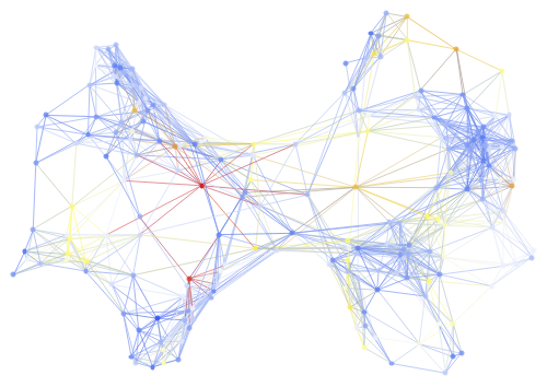
Kretschmann analogue estimated with Cubic Mean Deviation on the left and the former Kretschmann scalar calculated with the coordinates of the vertices on the right for a 300 vertex hypergraph (r = 3):
Row[ColorGraph[graphinf3,Transpose[{pointsif3,#}],500,3]&/@{CMDi3f300,krif3}]
Out[]=
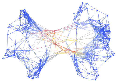
Kretschmann analogue estimated with Cubic Mean Deviation on the left and the former Kretschmann scalar calculated with the coordinates of the vertices on the right for a 300 vertex hypergraph (r = 6):
In[]:=
Row[ColorGraph[graphinf3,Transpose[{pointsif3,#}],500,3]&/@{CMDi6f300,krif3}]
Out[]=
Calculating the correlation coefficient and the correlation test for radii 3 and 6:
ρ
0
In[]:=
cρ3if3=Correlation[CMDi3f300,krif3]
Out[]=
-0.0123379
In[]:=
CP3if3=CorrelationTest[Transpose[{CMDi3f300,krif3}],cρ3if3]
Out[]=
0.403107
In[]:=
cρ6if3=Correlation[CMDi6f300,krif3]
Out[]=
-0.0129549
In[]:=
CP6if3=CorrelationTest[Transpose[{CMDi6f300,krif3}],cρ6if3]
Out[]=
0.79855
Taking all the correlation test results for the 5 graphs:
In[]:=
ListPlot[{{CP3if1,CP3if2,CP3if3,CP3if4,CP3if5},{CP6if1,CP6if2,CP6if3,CP6if4,CP6if5}},DataRange{100,500},PlotLegends{"r=3","r=6"},FrameLabel{"Statistics","Statistics"},GridLinesAutomatic,FrameTrue,ImageSizeLarge,LabelStyle->Directive[Bold,10]]
Out[]=
We notice a clear indication of convergence for the Flamm’s hyperboloid case.
Concluding remarks
Concluding remarks
The results seem to indicate an unstable convergence as the point density increases. However, more hypergraph points are needed in order to obtain conclusive results.
The Kretschmann analogue estimated with the Cubic Mean Deviation on the 200 vertex hyperboloid hypergraph for radius 3 seems very promising in comparison to previous attempts done with the absolute mean deviation, but more results are needed especially to observe a convergence for the hypergraphs produced by sprinkling points within a hyperboloid.
The Flamm’s paraboloid case at low resolution does not show a clear qualitative coincidence between the estimated and the analytical Kretschmann scalar, but there is a more noticeable convergence as the number of vertex increases.
An immediate step to extend the project would be to perform higher resolution tests with more vertex points to perform a new convergence analysis of the Kretschmann estimates to true values with respect to metrics. Another important step is to attempt to prove an analytical relationship between values in the continuum limit.
p
L
Keywords
Keywords
◼
Kretschmann Scalar
◼
General Relativity
◼
Causal Sets
Acknowledgment
Acknowledgment
Foremost, I would like to thank my mentor, Jonathan Gorard for his patience, enthusiasm, disposition to discuss this project, and carefully proofreading of this document before submission. I would like to thank Cameron Beetar for the rapid responses to doubts and for providing extra background material. I could not ask for better mentors for the WSS. Both have given us a really enjoyable experience during these four weeks.
Also, I would like to thank everyone in our mentor group for making the summer school so entertaining- Joana Teixeira, Jan Chojnacki, Julia Dannemann-Freitag, Salvo Vultaggio, and Vlad Kuchkin. I would like to thank Stephen Wolfram for his sharing his time and knowledge with us during this school. Finally, I would like to thank Erin Cherry, TAs, and all the admin team for the successful organization and their availability to enjoy this experience.
I may also thank Johann Quenta for the crash course on manifolds and metrics.
References
References
◼
[1] Hawking, Stephen, and George F. Ellis. The large scale structure of space-time. Cambridge England New York: Cambridge University Press, 1973.
◼
[2] Henry, Richard Conn. 2000. “Kretschmann Scalar for a Kerr-Newman Black Hole.” The Astrophysical Journal 535 (1): 350–53. https://doi.org/10.1086/308819.
◼
[3] Gorard, Jonathan. 2020. “Some Relativistic and Gravitational Properties of the Wolfram Model”. https://www.wolframcloud.com/obj/wolframphysics/Documents/some-relativistic-and-gravitational-properties-of-the-wolfram-model.pdf
◼
[4] Ryder, Lewis H. Introduction to general relativity. Cambridge, UK New York: Cambridge University Press, 2009.
Code
Code