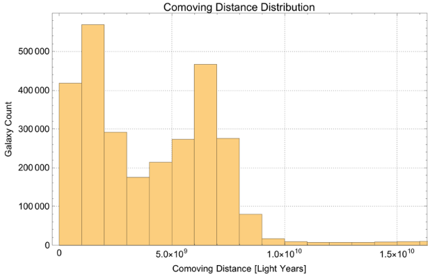
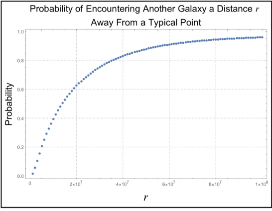
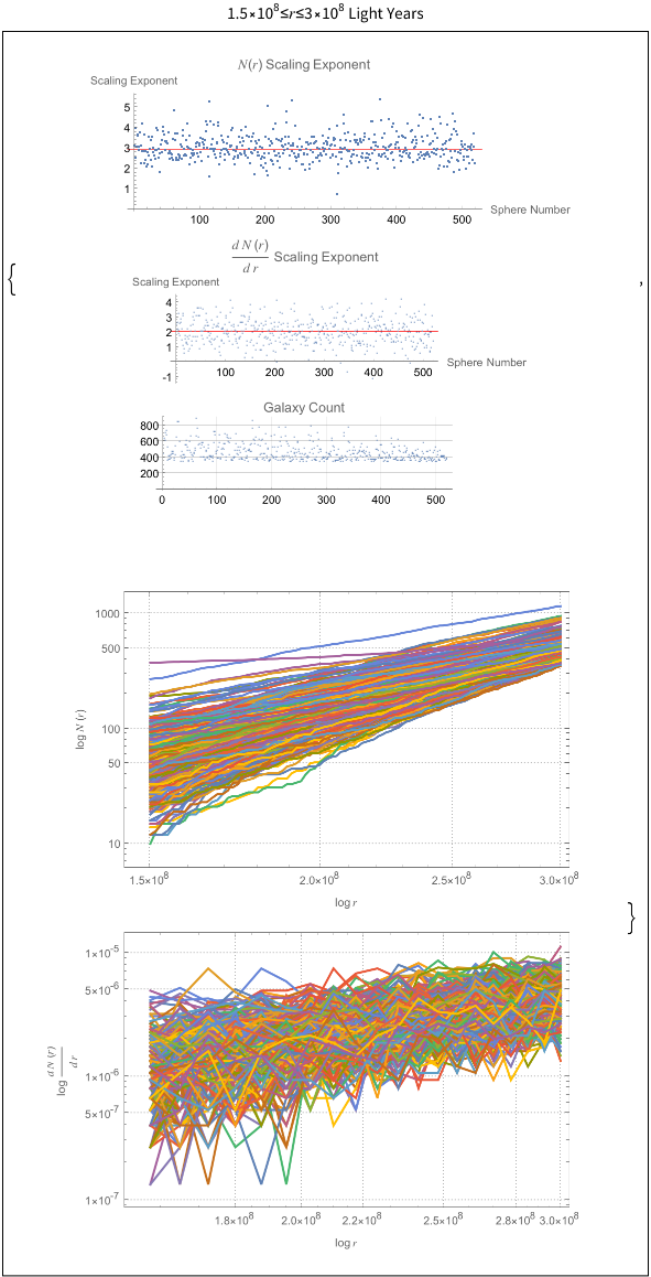
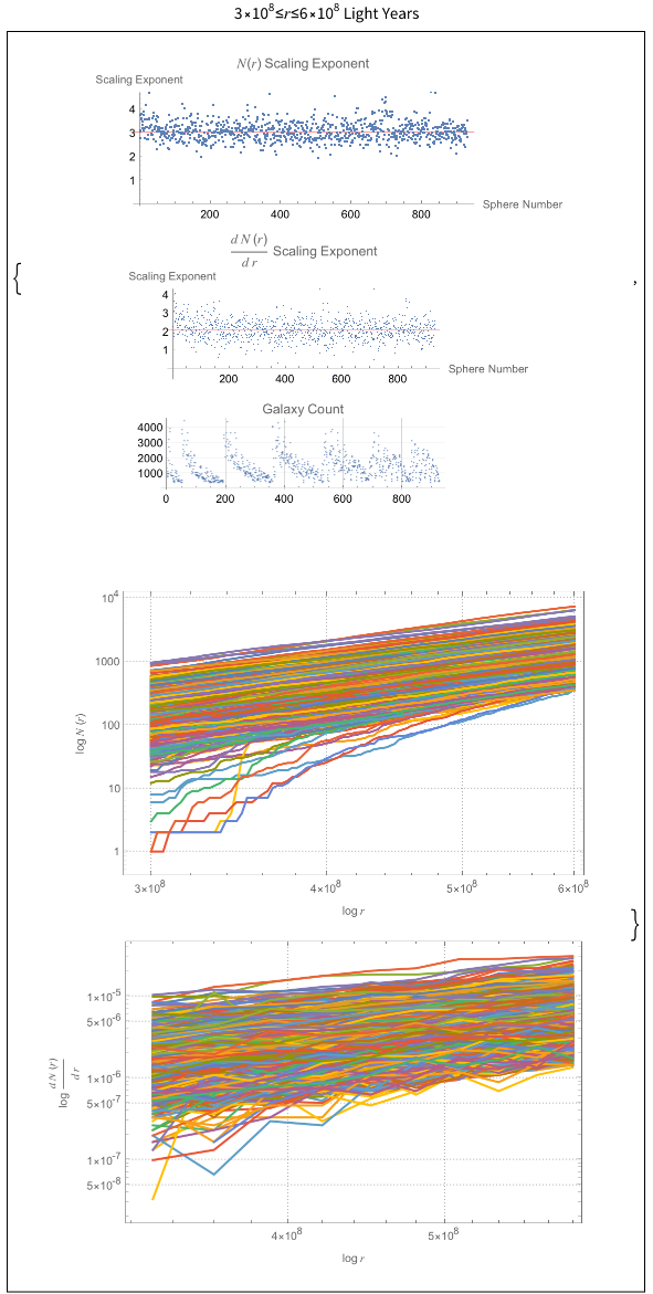
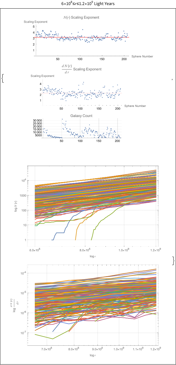
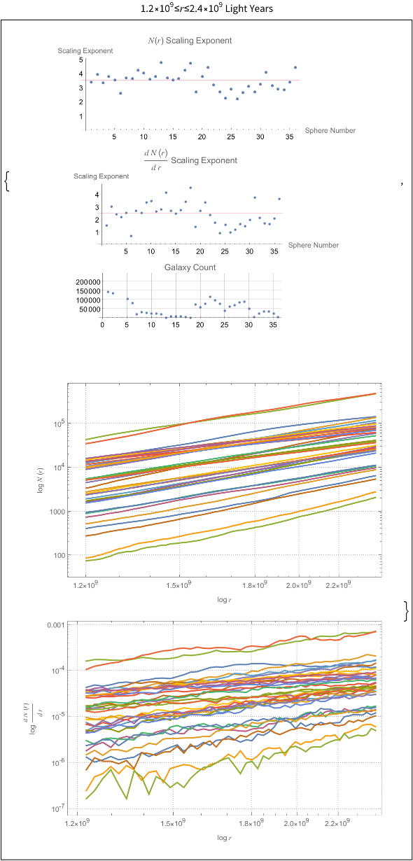
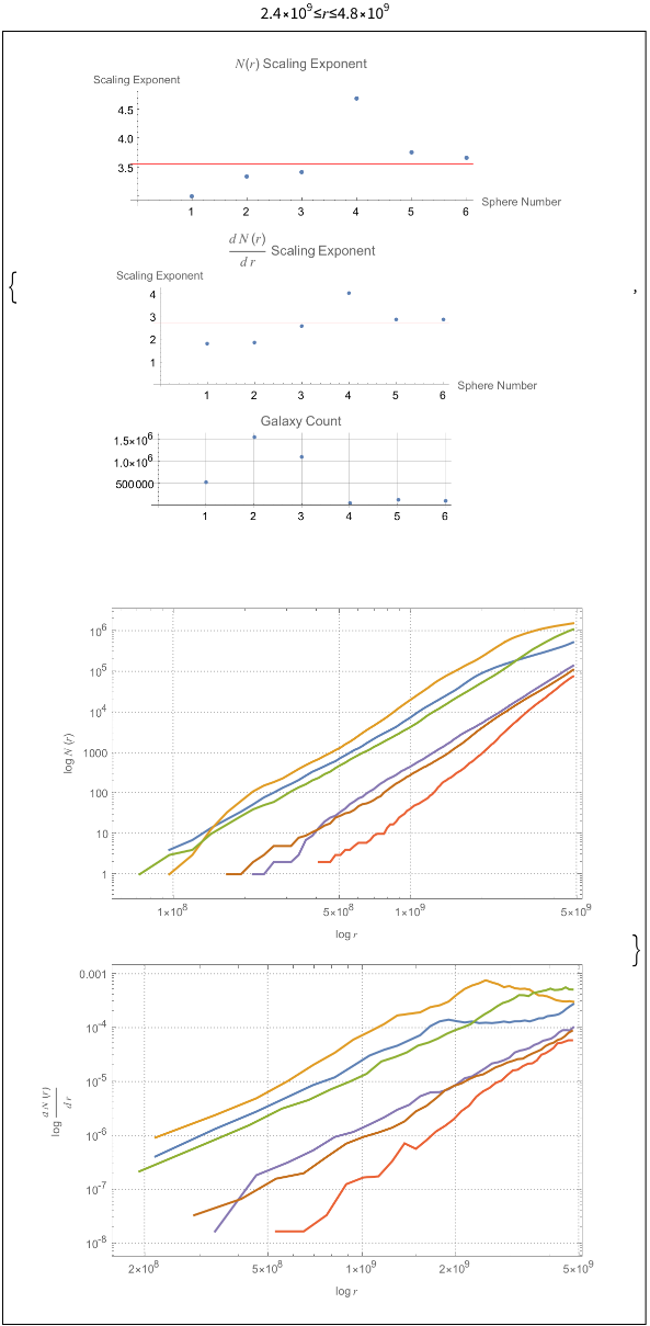
The power law scaling of galaxy distributions sourced from HyperLEDA are measured using growing spherical shells. Measurements are performed in isolation as well as in a three dimensional grid configuration using hundreds of shells. It is found that the power law exponent is not uniform in isolation, but will always cluster around a particular value when repeated enough times using a sphere radius that is not too large. The results found are unsurprising, and typically center around the expected values of
N(r)∝
3
r
, and
dN(r)
dr
∝
2
r
, but exceed these values for
r>1.2
9
10
light years. The explanation for such a deviation can likely be explained by the introduction of large scale structures in the spheres causing a lack of uniformity in the distributions.

Introduction

This project is an investigation into how collections of galaxies scale with volume. If we were to place a massive sphere in space so that it contains many galaxies inside of it, what type of power law does the number of galaxies contained by the sphere’s radius obey as we allow the sphere to grow? Common sense says that
N(r)∝
3
r
, but what if this is not the case? If the possibility exists that the early universe was born from fractional dimensional space, then any region found with non-cubic scaling could be of potential interest to researchers. The goal of this project is to provide a method for performing wide-scale searches for regions that exhibit this type of behaviour, and to identify any other possible explanations that may be causing it.

Data Acquisition and Reduction

The HyperLEDA Database

All of the data used in this project was sourced from HyperLEDA, a massive database containing astrophysical parameters for confirmed galaxies, sourced from multiple surveys and academic publications. The database is maintained through a collaboration between Lyon Observatory, France, and The Special Astrophysical Observatory, Russia.
​
For each galaxy in the database, there are multiple measurements available to use. For this project, the data was downloaded using their SQL Query form, requesting the mean of these measurements for all galaxies and quasars, including relevant parameters like redshifts and coordinates in different frames. Because the database is so large and computationally expensive to import, I imported it a single time as a CSV file and then immediately exported it again to an .mx file. The original file I used can be downloaded here from Google Drive, or you can generate your own file using the SQL form. I only requested the parameters that I needed for this project, but there are tons of other interesting things you can get from there. Here we load all of the coordinates in the galactic frame.
In[]:=
galaxies=Import["/Users/lukewriglesworth/galaxies.mx"];​​header={"objname","al1950","de1950","al2000","de2000","l2","b2","sgl","sgb","v","mod0","modbest"};​​longitude=galaxies[[All,6]];​​latitude=galaxies[[All,7]];

Calculating Distances to Each Galaxy

Redshifts

There is no column for distance in the CSV file because it is assumed you will do this step yourself based on the range of coordinates your project requires. For this project I calculate distances using redshifts, as other possible methods would only be applicable to a small fraction of the coordinates.
In[]:=
v=galaxies[[All,10]];​​c=UnitConvert[
c
,"Kilometers"/"Seconds"];​​redShifts=v/QuantityMagnitude@c;
I first start with the mean heliocentric radial velocity, indicated by the letter
v
in the header row. Then we use the formula
v=cz
to calculate the redshifts of each galaxy.

Comoving Distance

In cosmology there are two ways of talking about distance, comoving distance and proper distance. Proper distance is the type of distance you are familiar with, which is valid in a reference frame where two coordinate measurements happen at the same cosmological time. When we make a measurement of a galaxy from earth, it is not a true representation of where the galaxy is at the time we make our measurement due to the expansion of the universe and the delay caused by the finite speed of light. The easiest way to solve this problem is to define a new coordinate system that expands along with the universe, which is how we define comoving distance. At the current time, comoving distance and proper distance are defined to be the same, but they will differ in the past in future. The animation below from Wikipedia does a great job at showing how comoving coordinates behave.
Out[]=
Source: https://commons.wikimedia.org/wiki/File:Cosmos-animation_Lambda-CDM.gif

Removal of Blueshift Galaxies

Since my method of choice for distance calculation relies on all the galaxies having a measured redshift, any blueshift galaxies must be removed to prevent nearby galaxy positions from becoming distorted.
In[]:=
redShiftStepFunction=UnitStep@redShifts;​​fractionBlueShift:=(Length@redShifts-Total@redShiftStepFunction)/Length@redShifts;​​fractionBlueShift
Out[]=
97
2868898
We have 97 blueshift galaxies. We won’t miss them out of 2.9 million. Here I pick out the latitudes, longitudes and redshifts that are associated with galaxies that have redshifts greater than zero and reassign them to the redShifts variable:
In[]:=
latitude=Pick[latitude,redShiftStepFunction,1];​​longitude=Pick[longitude,redShiftStepFunction,1];​​redShifts=Pick[redShifts,redShiftStepFunction,1];​​Length@latitude==Length@longitude==Length@redShifts​​fractionBlueShift
Out[]=
True
Out[]=
0

Comoving Distance using the LambdaCDM Cosmological Model

To calculate comoving distances, I use the Lambda Cold Dark Matter cosmological model along with three specific parameters mentioned by the HyperLEDA documentation. The parameters I set are a specific value for the Hubble constant,
H
0
, as well as
Ω
M
and
Ω
λ
. These parameters control the rate of expansion, non-relativistic matter density, and the dark energy density used in the model. The Wolfram Language has a great function called UniverseModelData that makes this very easy:
In[]:=
hyperLEDAParameters={"LambdaCDM",<|"HubbleH0"->Quantity[70,"Kilometers"/("Seconds"*"Megaparsecs")],"OmegaMatter"->0.27`,"OmegaLambda"->0.73`|>};
In[]:=
d[z_]:=
UniverseModelData
[<|"Redshift"->z|>,"ComovingDistance",hyperLEDAParameters];​​comovingDistance=Parallelize[d[#]&/@redShiftsFiltered];

Visualization of the Galaxies

Redshift Colormapping

To make the visualizations nicer, we can map the galaxies to a corresponding color based on their redshifts. I adjusted the contrast of the color mapping to make it look nicer, so it is not 100 percent accurate. Its primary purpose is to quickly show which galaxies are nearby and which are distant.
gammaCorrection[x_,γ_]:=x^(1/γ);​​scaling=gammaCorrection[#,4]&;​​minRedShift=Min[redShifts];maxRedShift=Max[redShifts];​​redShiftNormalized=Rescale[redShifts,{minRedShift,maxRedShift}];​​colorFunction=Blend[{Blue,Red},scaling[#]]&;​​plotColors=colorFunction/@redShiftNormalized;​​barLegend=BarLegend[​​{colorFunction,{Min[redShiftNormalized],Max[redShiftNormalized]}},​​LegendLabel->Style["Redshift",23],​​"Ticks"->{-1,0,1},​​"TickLabels"->{Max[redShifts],Min[redShifts]},​​"TickSide"->Right,​​"TickLengths"->10,​​"TicksStyle"->Directive[Black,20]​​];

A Two Dimensional Galaxy Map

Now we have everything needed to visualize the data. I am using GeoGraphics here for the Aitoff map projection.
In[]:=
twoDimCoordinates=Thread[{latitude,longitude}];​​ticksLatitude=Table[{iDegree,iDegree},{i,-180,180,30}];​​ticksLongitude=Table[{iDegree,iDegree},{i,-75,75,15}];​​twoDimMap=Legended[GeoGraphics[​​{PointSize[0.00001],Point[GeoPosition[twoDimCoordinates],VertexColors->plotColors],PlotStyle->{".",Tiny}},​​GeoProjection->"Aitoff",​​GeoRange->{All,All},​​GeoGridLines->Automatic,​​GeoGridLinesStyle->White;​​GeoBackground->Black,​​AxesStyle->White,​​TicksStyle->{{White,10},{White,10}},​​Axes->{True,True},​​Ticks->{ticksLatitude,ticksLongitude},​​PlotLabel->Style["Galaxies viewed in Galactic Coordinates"]​​],barLegend];
Here I thread the coordinates together to make latitude and longitude pairs, and setup a custom range of tick marks to match the coordinate system.
Click the image to see it in full resolution:

Conversion to Cartesian Coordinates

We currently have the galaxy positions in spherical coordinates, which will be very challenging to use for the type of analysis we want to do. Let’s convert to Cartesian coordinates before going any further.
sphericalCoordinates=Thread[{QuantityMagnitude@comovingDistance,longitude*Pi/180,latitude*Pi/180}];​​cartesianMapping=CoordinateTransformData[{"Spherical"->"Cartesian"},"Mapping"];​​cartesianCoordinates=cartesianMapping/@sphericalCoordinates;

A Three Dimensional Galaxy Map

We can now plot the galaxy positions in three dimensional Cartesian coordinates. I am using Graphics3D here because I found the performance to be a bit better when plotting so many points:
threeDimMap=Labeled[Graphics3D[{​​PointSize[0.001],Point[cartesianCoordinates,VertexColors->plotColors],​​PlotStyle->{".",Tiny}​​},​​Background->Black,​​Ticks->Automatic,​​Axes->True,​​AxesStyle->White,​​Boxed->True,​​AxesLabel->{"Light Years","Light Years","Light Years"}​​],barLegend,Right];
Click the image to see it in full resolution:
Out[]=
At this point we now have a working model of the universe ready to go, and can start working towards the actual goal of the project.

Bonus Visualization!

We didn’t go any further in this direction, but this is the result of running the DBSCAN clustering algorithm on the plot above. I had to include it because it’s awesome.
Click the image to see it in full resolution:

Measuring Power Law Scaling in Galaxy Distributions

Methodology

The basic idea behind the method I use is that if we have a uniform distribution of particles and we place a sphere inside this distribution, the number of particles within the sphere at any radius will grow proportionally to the sphere’s radius cubed:
In the case of galaxies, we don’t know exactly what this exponent will be, even though it is expected to be three. The way I answer this question is by placing many overlapping spheres in a three dimensional grid, calculating
from half the sphere’s radius up to its maximum radius in each one of the spheres. The reason multiple spheres are used is because single measurements do not tell us much. You may notice in the next section’s demonstration that even with dense, randomly generated points in a tiny sphere there are considerable variations in the measurements when running the code multiple times. The distribution of galaxies on a large scale may look uniform at first glance because we have so much data, but the effects of gravitational clustering can cause a large difference in results just by moving the sphere a tiny bit. By surveying a large number of galaxies at once, we can get an overall sense of what number these measurements are centered around.​Another quantity of interest we can easily calculate is the differential number count,
, which tells us the number of new galaxies encountered for a corresponding change in
. In the code, the differential number count is calculated by finding the differences in
for larger differences in
than where
is calculated. This allows the derivative to still be approximated even while
remains constant on a smaller length scale.

Measuring Power Law Scaling in a Single Sphere

The following code performs measurements of the scaling exponents for
,
, and also returns a visualization of what it is doing. The scaling exponents are calculated by fitting a line to the functions on a logarithmic scale to get their slopes. The demonstration here is generated using randomly generated coordinates.

Click here to see the code and a visualization:


Extension to Multiple Spheres.

Starting with the code shown above, we can easily extend it to measure over a 3D rectangular region filled with overlapping spheres. In order to run this you will need to remove searchVisualization from the return list of the previous function, as it will probably crash your computer generating a visualization for each individual sphere. The function below returns its own visualization for the entire grid, and there is also a function to quickly plot results. The median of the measurements is shown as a red line in the plots, and is also output as an Echo.

Click here to see the code and a visualization:


Performing Real Measurements

We now have all the tools in place to start doing actual measurements on the data. Since the grid measurement function takes a range of boundaries to setup the grid, the first step is to figure out what those are going to be. I start by plotting the cross section of the dataset.
In[]:=
plotCrossSection[coordinates_]:=Module[​​{},​​Framed[​​GraphicsRow[{​​ListPlot[Thread[{coordinates[[All,1]],coordinates[[All,2]]}],AxesLabel->{"X","Y"},PlotLabel->"XY Plane",PlotStyle->{".",Black,Tiny},AspectRatio->1,Frame->True,FrameTicks->All,PlotRange->Full],​​ListPlot[Thread[{coordinates[[All,2]],coordinates[[All,3]]}],AxesLabel->{"Y","Z"},PlotLabel->"YZ Plane",PlotStyle->{".",Black,Tiny},AspectRatio->1,Frame->True,FrameTicks->All,PlotRange->All],​​ListPlot[Thread[{coordinates[[All,1]],coordinates[[All,3]]}],AxesLabel->{"X","Z"},PlotLabel->"ZX Plane",PlotStyle->{".",Black,Tiny},AspectRatio->1,Frame->True,FrameTicks->All,PlotRange->All]​​}]​​]​​];
In[]:=
plotCrossSection[cartesianCoordinates]
Based on the plot above, we are most limited in the XY plane. I will select a large region in the upper right quadrant. The function below plots the cross section along with a rectangle in each plane to help confirm your choice of boundaries.
In[]:=
plotCrossSectionRegion[coordinates_,{xMin_,xMax_},{yMin_,yMax_},{zMin_,zMax_}]:=Module[​​{},​​Framed[​​GraphicsRow[{​​Graphics[​​{Black,PointSize[0.0001],ParallelMap[Point[#]&,Thread[{coordinates[[All,1]],coordinates[[All,2]]}]],​​Red,Opacity[0.5],Rectangle[{xMin,yMin},{xMax,yMax}],​​AspectRatio->Automatic}],​​Graphics[​​{Black,PointSize[0.0001],ParallelMap[Point[#]&,Thread[{coordinates[[All,2]],coordinates[[All,3]]}]],​​Red,Opacity[0.5],Rectangle[{yMin,zMin},{yMax,zMax}],​​AspectRatio->Automatic}],​​Graphics[​​{Black,PointSize[0.0001],ParallelMap[Point[#]&,Thread[{coordinates[[All,1]],coordinates[[All,3]]}]],​​Red,Opacity[0.5],Rectangle[{xMin,zMin},{xMax,zMax}],​​AspectRatio->Automatic}]​​}]​​]​​]
In[]:=
plotCrossSectionRegion[cartesianCoordinates,{0.25*10^9,4*10^9},{2*10^9,7*10^9},{-6*10^9,6*10^9}]
The intention here is to perform repeated measurements on the same region but at different ranges of
to see how the exponents may change. The grid measurement function will redistribute the locations of the spheres to fill the box, so we only need to worry about setting the radii and the step size
dr
at which
is calculated. I set up my measurements to use 100 steps of
for each sphere.​To get a rough idea of the minimum radius to set, we can generate the nearest neighbour probability distribution. This shows the probability of encountering another galaxy at a given radius from a typical point:
In[]:=
neighbourFunction=NearestNeighborG[cartesianCoordinates];​​points=Range[10^6,10^8,10^6];
In[]:=
probabilities=ParallelMap[neighbourFunction,points];
In[]:=
ListPlot[Thread[{points,probabilities}],PlotTheme->"Detailed",PlotLabel->Style["Probability of Encountering Another Galaxy a Distance
From a Typical Point",Black,20]]
The main factors we are considering here are the need for a minimum number of galaxies per sphere, and if we compute too many spheres we also run the risk of crashing the computer. Based on the nearest neighbour distribution and a few trial measurements, I set the smallest scale measurement to be between
and
light years. This is obviously not that small, and that is because my laptop couldn’t handle going any smaller. I may update this post later with additional galaxies and smaller scale measurements.
In[]:=
measurementSmallSpheres=ballVolumeScalingGrid[3*10^8,{0.25*10^9,4*10^9},{2*10^9,7*10^9},{-6*10^9,6*10^9},cartesianCoordinates,1.5*10^6];​​measurementSmallSpheres=Select[measurementSmallSpheres,Length[#]>=4&];
»
Inner Radius1.5×
8
10
»
Outer Radius3.×
8
10
In[]:=
Labeled[plotGridMeasurement[measurementSmallSpheres],"
Light Years",Top]
»
N(r) Median Exponent2.94034
»
dN(r)/dr Median Exponent2.00344
Out[]=
Here the results are pretty much as I would expect. We have a pretty large spread between individual exponents, but the results are still centered around 3 and 2 for
and
. Next I setup the next measurement such that the inner radius becomes the outer radius of the previous measurement, continuing like this for all subsequent measurements.
In[]:=
measurementMediumSpheres=ballVolumeScalingGrid[6*10^8,{0.25*10^9,4*10^9},{2*10^9,7*10^9},{-6*10^9,6*10^9},cartesianCoordinates,3*10^6];​​measurementMediumSpheres=Select[measurementMediumSpheres,Length[#]>=4&];
»
Inner Radius3.×
8
10
»
Outer Radius6.×
8
10
In[]:=
Labeled[plotGridMeasurement[measurementMediumSpheres],"
Light Years",Top]
»
N(r) Median Exponent3.02735
»
dN(r)/dr Median Exponent2.0935
Out[]=
This measurement is extremely similar to the previous one, but with more uniform slopes and values even closer to 3 and 2.
In[]:=
measurementLargeSpheres=ballVolumeScalingGrid[1.2*10^9,{0.25*10^9,4*10^9},{2*10^9,7*10^9},{-6*10^9,6*10^9},cartesianCoordinates,6*10^6];​​measurementLargeSpheres=Select[measurementLargeSpheres,Length[#]>=4&];
»
Inner Radius6.×
8
10
»
Outer Radius1.2×
9
10
In[]:=
Labeled[plotGridMeasurement[measurementLargeSpheres],"
Light Years",Top]
»
N(r) Median Exponent3.17925
»
dN(r)/dr Median Exponent2.23748
Out[]=
At this size of
we have begun to slightly exceed the expected values, with 3.17925 for
and 2.23748 for
.
In[]:=
measurementLargerSpheres=ballVolumeScalingGrid[2.4*10^9,{0.25*10^9,4*10^9},{2*10^9,7*10^9},{-6*10^9,6*10^9},cartesianCoordinates,1.2*10^7];​​measurementLargerSpheres=Select[measurementLargerSpheres,Length[#]>=4&];
»
Inner Radius1.2×
9
10
»
Outer Radius2.4×
9
10
In[]:=
Labeled[plotGridMeasurement[measurementLargerSpheres],"
Light Years",Top]
»
N(r) Median Exponent3.54461
»
dN(r)/dr Median Exponent2.47614
Out[]=
We are now seeing a huge deviation from 3 and 2, with 3.54461 for
and 2.47614 for
. Let’s do one more measurement just to see what happens.
In[]:=
measurementLargestSpheres=ballVolumeScalingGrid[4.8*10^9,{0.25*10^9,4*10^9},{2*10^9,7*10^9},{-6*10^9,6*10^9},cartesianCoordinates,2.4*10^7];​​measurementLargestSpheres=Select[measurementLargestSpheres,Length[#]>=4&];
»
Inner Radius2.4×
9
10
»
Outer Radius4.8×
9
10
In[]:=
Labeled[plotGridMeasurement[measurementLargestSpheres],"
",Top]
»
N(r) Median Exponent3.55451
»
dN(r)/dr Median Exponent2.72827
Out[]=
We can’t fit many more spheres in the box, so I think it’s time to stop. One thing I do notice that’s unusual here is that the slope for
is practically unchanged from the previous measurement, and the slope of the derivative has increased even higher to 2.72827.

Can We Measure the Entire Dataset?

It is definitely possible to do measurements on the entire database in chunks. Even though I don’t have enough time to measure the rest of the database in a similar style, it is still possible to survey the entire database using just a single sphere placed at the origin. This is very computationally intensive, but I managed to approximate
using a large step size giving us 1000 points.
In[]:=
everythingMeasurement=ballVolumeScaling[3*10^10,{0,0,0},cartesianCoordinates,3*10^7];
In[]:=
ListPlot[everythingMeasurement[[4]],PlotRange->All,PlotTheme->"Detailed",PlotLabel->Style["
Over the Entire Dataset",20],FrameLabel->{"
","
"},FrameStyle15,PlotStyle->{".",PointSize[0.004]}]
Out[]=
Let’s check this out on a log-log plot:
In[]:=
everythingMeasurement[[1]]​​ListPlot[everythingMeasurement[[4]],PlotRange->All,PlotTheme->"Detailed",PlotLabel->Style["
Over the Entire Dataset",20],FrameLabel->{"
","
"},FrameStyle15,PlotStyle->{".",PointSize[0.003]},ScalingFunctions->{"Log","Log"},PlotRange->All]
Out[]=
It looks like there are different scaling exponents for different ranges of
. Let’s look at each one and see what they are:
In[]:=
fitSlopeSection[measurement_,x1_,x2_]:=Module[​​{plot,logPoints,linearFit,x},​​logPoints=Log[measurement[[4,Nearest[measurement[[4,All,1]]->"Index",x1][[1]];;Nearest[measurement[[4,All,1]]->"Index",x2][[1]]]]];​​linearFit=LinearModelFit[logPoints,{x,1},x];​​plot=Show[​​Plot[linearFit[x],{x,Log[x1],Log[x2]},PlotTheme->"Detailed",FrameLabel->{"
","
"},PlotLegends->{StringJoin["Slope: ",ToString@linearFit["BestFitParameters"][[1]]]},ScalingFunctions->{"Linear","Linear"}],​​ListPlot[logPoints,PlotStyle->{".",Red},PlotTheme->"Detailed",ScalingFunctions->{"Linear","Linear"}]​​];​​plot​​]​​section1=Labeled[fitSlopeSection[everythingMeasurement,3*10^7,1*10^9],"
Light Years",Top]​​section2=Labeled[fitSlopeSection[everythingMeasurement,3*10^7,9*10^7],"
Light Years",Top]​​section3=Labeled[fitSlopeSection[everythingMeasurement,9*10^7,2*10^8],"
Light Years",Top]​​section4=Labeled[fitSlopeSection[everythingMeasurement,1.8*10^8,5*10^8],"
Light Years",Top]​​section5=Labeled[fitSlopeSection[everythingMeasurement,5.8*10^9,6.6*10^9],"
Light Years",Top]​​
Out[]=
Although the results in this section seem to conflict with what was observed using the grid measurement method using multiple spheres, we must remember that
was approximated on quite a large interval here. Even though 1000 sample points seems like alot, on the scale of this dataset this amounts to a distance of 30 million light years between measurements, so we can expect to see significant errors when checking the slopes of small sections of
. These plots were generated from just a single measurement as well, and are therefore not comparable to the previous results, which also showed large variations between single measurements. As an estimate of the scaling exponent for
these plots are not of much use, but are certainly helpful at showing the distribution of galaxies at different distances from the origin.

Conclusion

The main conclusion I found is that the scaling exponent for galaxy distributions can not be accurately predicted on a small, individual measurement basis, as a tiny change in a sphere’s location typically alters the exponent by at least
. I was expecting this to be the case, since galaxy distributions are not uniform due to gravitational clustering and large scale structures. I worked around this issue by performing continuous measurements over large grid regions and observing trends instead of focusing on single measurements. I found that the scaling exponents over large regions always clustered around a specific number that is somewhat correlated with the sphere radii chosen to fill the grid. For measurements with radii ranging from
to
light years, the results for
and
centered around what would be expected, 3 and 2. However, for radii higher than that I found a notable increase in the exponents, reaching maximum values of 3.55451 for
and 2.72827 for
. These results are unsurprising to me, as filling the grid with larger spheres will increase the probability of including inhomogeneous regions in the measurement.

Future Work

It’s important to emphasize at this point that this project is just an initial exploratory effort, and is not anywhere near rigorous enough to make claims about the dimensionality of the regions we measured. Our goal here was to provide an excellent starting point for future researchers who might be interested in the same question as us, and I think we were very successful in that goal. There are many features that still need to be implemented in the code that would improve the clarity of results. The most obvious is the inclusion of uncertainties and residuals of the linear fits. We are essentially performing only a single measurement and calculation, so the error propagation and would be very minimal. These improvements will give a much cleaner look into how well the code is performing, and would help us filter out bad measurements that may be skewing the results. The code also needs significant optimization to reach its full potential. Right now we are measuring each overlapping sphere individually while ignoring the results of neighbouring spheres. If we could figure out a way to share some information between the spheres it would dramatically improve the speed of measurement.
​
The last improvement is in regards to the data itself. By limiting ourselves to only HyperLEDA coordinates, we are including only a tiny fraction of the galaxies in the universe. Although HyperLEDA includes only confirmed galaxies, the usage of less studied, potential galaxies would likely be helpful. This is an extremely data heavy project, and the more data we can incorporate the better. This would of course require much more computation power, and is why I didn’t do this in the first place.

Acknowledgments

I would like to give a huge thank you to both my mentors, Sotiris Michos and Alejandra Ortiz Duran. They spent many hours with me during the school, and I would not have been able to complete the project without their help (and animating skills). I would also like to thank Stephen Wolfram for turning my very foggy idea into something I could actually get done in a couple weeks, and also for giving me very good advice during the midpoint meeting.
​
I would also like to thank my grandma, Diane Wright, who paid for me to attend the Summer School, there would definitely be no project without her. Also thank you to my wife Mariam who let me abandon her for three weeks.

Cite This Notebook

“Searching for indications of fractional dimensions”
by Luke Wriglesworth​
​https://community.wolfram.com/groups/-/m/t/3210754