Before joining Wolfram I spent roughly eight years immersed in numerical computation. Once here, I discovered the power of arbitrary-precision arithmetic and its surprising connection to chaos theory: a toolset I had never made use of before. The experience led me to give a talk on Wolfram’s precision framework at the Wolfram Technology Conference and to weave these ideas into the numerics courses I teach at the Wolfram Summer School and subsequent conferences. Delving into precision has even shed light on some of my deeper philosophical questions. I am sharing that journey here in the hope that it may spark similar insights for others.
On the Razor’s Edge of Precision
On the Razor’s Edge of Precision
1. Why should I care about “Precision”?
1. Why should I care about “Precision”?
When we are doing computations with relatively small (say less than ) or large numbers (say greater than ) with the default arithmetic our machine uses for everyday floats, round-off error can snowball until the answer loses meaning.
-5
10
5
10
Consider this simple computation - Sin of a large number:
In[]:=
Sin[10^30.]
Out[]=
0.00933147
In fact we get the same answer if we execute the command in C language - check it out here. However using Sign says something contradictory - Sin[10^30] is a negative number:
In[]:=
Sign[Sin[10^30]]
Out[]=
-1
Where did we go wrong? We could not derive an accurate value using the default machine precision arithmetic. Use arbitrary precision to get the correct result:
In[]:=
N[Sin[10^30],10]
Out[]=
-0.09011690191
2. The three numeric species
2. The three numeric species
1. Machine precision - the fast lane with hidden potholes
If the number of digits is 17 or less, or if it ends with a backtick - it is Wolfram Language (WL) considers it to be in machine precision. Examples:
{2.3(*2digits*),1.2345678901234567(*17digits*),1.2345678901234567890123456789012`(*32digitsbutendswithabacktick*)}
Check the interpretation using the function Precision:
In[]:=
Precision/@{2.3(*2digits*),1.2345678901234567(*17digits*),1.2345678901234567890123456789012`(*32digitsbutendswithabacktick*)}
Out[]=
{MachinePrecision,MachinePrecision,MachinePrecision}
In a computation, if the inputs are in machine precision, WL employs machine precision framework for the computation and the result is in machine precision: Machine precision in → machine precision out
In[]:=
2.3+1.5
Out[]=
3.8
In[]:=
Precision[%]
Out[]=
MachinePrecision
Machine precision computation is less accurate but faster. Error is not tracked during the computation.
2. Arbitrary precision - crank the dial yourself
If the number of digits is more than 17, it is considered to be in arbitrary precision. If the number of digits is less than or equal to 17, the precision can be specified using backtick or SetPrecision (and it is considered to be in arbitrary precision). Examples:
In[]:=
Precision/@{2.30000000000000000000,(*19zeros,21digits*)2.3`20,(*2digitsbutprecisionsetusingbacktick*)SetPrecision[2.34,20](*3digitsbutprecisionsetusingSetPrecision*)}
Out[]=
{20.3617,20.,20.}
Arbitrary precision framework is selected if the inputs are in arbitrary precision and the result follows similarly: Arbitrary precision in → arbitrary precision out
In[]:=
2.3`10+1.5`10
Out[]=
3.800000000
In[]:=
Precision[%]
Out[]=
10.
Arbitrary precision is more accurate but slower. Error is tracked.
3. Infinite precision - the exact end of the rainbow
Examples:
In[]:=
Precision/@{23/10,45,Pi}
Out[]=
{∞,∞,∞}
For this the computations are exact - no error to track:
In[]:=
2/3+10
Out[]=
32
3
In[]:=
Precision[%]
Out[]=
∞
3. Precision frameworks in numeric functions
3. Precision frameworks in numeric functions
Most of the numeric functions use MachinePrecision by default:
In[]:=
NIntegrate[1.5x^2Sin[x],{x,0,1}]
Out[]=
0.334866
In[]:=
Precision[%]
Out[]=
MachinePrecision
Use the option WorkingPrecision along with exact inputs to enforce ArbitraryPrecision:
In[]:=
NIntegrate[Rationalize[1.5]x^2Sin[x],{x,0,1},WorkingPrecision->20]
Out[]=
0.33486641322589909606
In[]:=
Precision[%]
Out[]=
20.
Here is a demo where MachinePrecision can lead to a totally incorrect answer.
deq1=[t]-x[t]-0.8y[t]+0.4;deq2=[t]2x[t]+1.0y[t]-x[t]*y[t]-0.2835;
′
x
2
y[t]
′
y
2
y[t]
In[]:=
sol1=NDSolve[{deq1,deq2,x[0.0]-0.000001,y[0.0]0.0},{x,y},{t,0.0,5000}];
Starting from the initial coordinates of , the plot is supposed to spiral inward - but computations show that it goes outward:
{x[0.0]==-0.000001,y[0.0]==0.0}
In[]:=
ShowParametricPlotEvaluate[{x[t],y[t]}/.sol1],{t,0.0,500},,ParametricPlotEvaluate[{x[t],y[t]}/.sol1],{t,0.0,20},
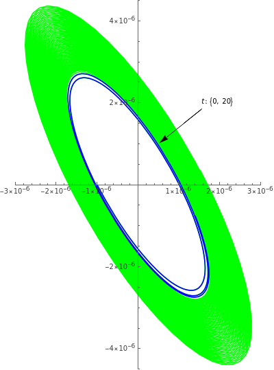
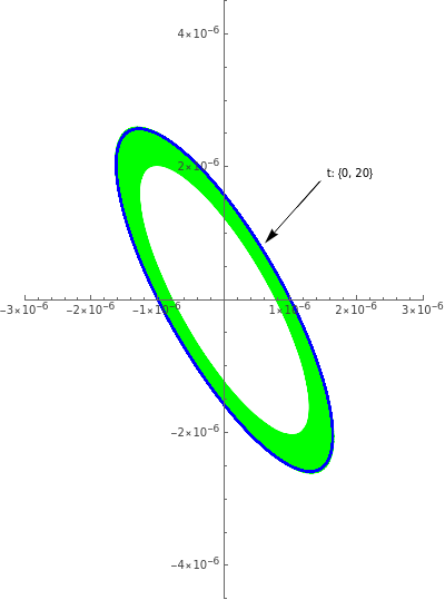
We get the expected behavior by using arbitrary precision framework:
deq1R=[t]-x[t]-Rationalize[0.8]y[t]+Rationalize[0.4];deq2R=[t]2x[t]+1y[t]-x[t]y[t]-Rationalize[0.2835];
′
x
2
y[t]
′
y
2
y[t]
sol2=NDSolve[{deq1R,deq2R,x[0]-Rationalize[0.000001],y[0]0},{x,y},{t,0,5000},WorkingPrecision50,MaxSteps200000];
ShowParametricPlotEvaluate[{x[t],y[t]}/.sol2],{t,0.0,5000},,ParametricPlotEvaluate[{x[t],y[t]}/.sol2],{t,0.0,500},
4. Numerical Conditioning vs. Unavoidable Machine Precision
4. Numerical Conditioning vs. Unavoidable Machine Precision
For large-scale, time-critical workloads e.g. think of refining a 5000 x 5000 fluid-dynamics grid every millisecond or inverting a million-by-million sparse matrix for a Monte-Carlo risk sweep, insisting on exact integers or even 50-digits arbitrary reals quickly becomes infeasible. Every extra digit roughly doubles the memory and time requirements. Also many high-performance kernels (FFT, BLAS) are designed only for machine floats. For example, a 3-D finite-difference Poisson solver that updates nodes per time step can run in under a second with machine doubles but, if we merely raise WorkingPrecision to 50, it would require about 14 GB of RAM for the field alone and would slow to minutes.
n=256³≈1.7×10⁷
Worse, some algorithms break entirely: exact rational arithmetic in a Krylov solver triggers exponential coefficient swell, exhausting memory before the first hundred iterations.
In practice, one pushes as far as the conditioning demands say a modest 10–20 guard digits and then accepts that the rest of the job belongs to optimized machine-precision computations, perhaps augmented by interval checks or residual testing to verify the accuracy.
Consider a large matrix:
In[]:=
mat1=;Dimensions[mat1]
Out[]=
{683,9}
Singular value decomposition in machine precision takes less than one tenth of a second:
In[]:=
SingularValueDecomposition[N[mat1]];//AbsoluteTiming
Out[]=
{0.0679088,Null}
20 digits arbitrary precision computation takes more than 30 times longer:
In[]:=
SingularValueDecomposition[SetPrecision[mat1,20]];//AbsoluteTiming
Out[]=
{2.40387,Null}
Exact computation freezes (aborted after an hour):
In[]:=
SingularValueDecomposition[mat1];//AbsoluteTiming
Out[]=
$Aborted
5. Exactitude as the Price of Truth
5. Exactitude as the Price of Truth
As we have seen, some mathematical systems are so delicately poised that a rounding error of only a few bits can send a computed trajectory veering into a completely different qualitative regime. Imagine trying to land a paper airplane on the head of a pin from a rooftop - being off by even a feather’s width sends it spiraling elsewhere.
Wolfram Language’s arbitrary and infinite precision frameworks therefore do double duty: they give us the numerical headroom to preserve each significant digit, and they propagate any residual uncertainty transparently so we know how faithfully the simulation mirrors the equations we wrote down.
This need for precision is a perfect lead-in to our next topic: chaos theory. In chaos theory, we study systems where tiny changes in the starting point, like a slight tweak to a number can lead to wildly different outcomes. Think of a weather forecast: a small change in today’s temperature reading could predict sunshine or a storm tomorrow.
Structured Uncertainty: Inside Deterministic Chaos
Structured Uncertainty: Inside Deterministic Chaos
Lawful Roots of Unpredictability
Lawful Roots of Unpredictability
Chaos is often mistaken for randomness, yet the hallmark of a chaotic system is strict determinism: every future state is fixed by the present one through an explicit set of equations. What makes these systems feel random is their sensitive dependence on initial conditions - the famous butterfly effect, in which a microscopic perturbation e.g. a “butterfly’s wing-beat” in São Paulo is exponentially magnified into a macroscopic outcome e.g. a tornado in Texas.
The numerical moral, foreshadowed in our precision section, is that even a rounding error in the fifteenth decimal place can catapult an orbit from placid regularity to wild oscillation. Long-term prediction fails not because the system is capricious, but because our numbers can never be specified with infinite exactness.

Figure 1: A visual metaphor of the butterfly effect: a single wing-beat unfurls into swirling streamlines that culminate in a tornado, illustrating how a microscopic nudge can cascade into macroscopic upheaval
Core ingredients of chaos
Core ingredients of chaos
Most systems that exhibit deterministic chaos share these mathematical features (read more about chaos in [1-3]):
◼
Nonlinearity: terms that multiply or compose the state variables break proportionality
◼
Stretching and folding (topological mixing): trajectories are continually pulled apart and re-injected into the same region of phase space
◼
Rapid growth of tiny differences: nearby trajectories diverge exponentially fast
Put together, these three ingredients lead to the classic hallmarks we associate with chaos:
◼
Flip-flop behaviour: A smooth change in a control knob suddenly makes the system jump from calm to wildly oscillating
◼
Fractal patterns: If we zoom in on the trail that a chaotic system traces, the wiggles never smooth out - you keep seeing smaller wiggles on top of larger ones, like a coastline viewed from higher and higher up
◼
Short prediction window: We can still forecast for a while (tomorrow’s weather is easier than next month’s), but sooner or later those runaway small errors drown out the signal
Let us look at some examples implemented in the Wolfram Language next.
Example 1 - Double Pendulum
Example 1 - Double Pendulum
A double pendulum consists of one pendulum attached to the end of another. Even though its equations of motion come straight from Newton’s laws and contain no randomness, the system is non-linear: each bob’s acceleration depends on products of sines, cosines, and the other bob’s velocity. That non-linearity gives the double pendulum a positive Lyapunov exponent - nearby trajectories in phase space separate exponentially fast. In practice this means that two setups differing by a millionth of a radian in one starting angle will swing identically for a short time and then diverge into utterly different, seemingly unpredictable dances.
In[]:=
Clear["Global`*"]
In[]:=
(*Parameters*)m1=m2=1.;(*massesofthebobs*)l1=l2=1.;(*lengthsofthearms*)g=9.81;(*constantofgravity*)tmax=25.;(*integrationhorizon*)θ10=π/2;(*initialangleoffirstarm*)θ20=π/2;(*initialangleofsecondarm*)θ̇10=θ̇20=0.;(*bothstartfromrest*)δ=10^-6;(*tinyperturbationofθ1(0)*)(*Differential-equationsolver*)ClearAll[solvePendulum]solvePendulum[θ1_,θ2_]:=Module{θ1f,θ2f,eqns},eqns=(m1+m2)l1θ1f''[t]+m2l2θ2f''[t]Cos[θ1f[t]-θ2f[t]]+m2l2θ2f'[t]^2Sin[θ1f[t]-θ2f[t]]+g(m1+m2)Sin[θ1f[t]]==0,m2l2θ2f''[t]+m2l1θ1f''[t]Cos[θ1f[t]-θ2f[t]]-m2l1θ1f'[t]^2Sin[θ1f[t]-θ2f[t]]+m2gSin[θ2f[t]]==0,θ1f[0]==θ1,θ2f[0]==θ2,θ1f'[0]==θ̇10,θ2f'[0]==θ̇20;NDSolveValue[eqns,{θ1f,θ2f},{t,0,tmax},AccuracyGoal->12,PrecisionGoal->12,Method->"StiffnessSwitching",MaxStepSize->5*^-4,MaxSteps->∞]solA=solvePendulum[θ10,θ20];solB=solvePendulum[θ10+δ,θ20];(*Cartesiancoordinatesofthesecondbob*)pos2[sol_][tt_]:=With[{θ1=sol[[1]][tt],θ2=sol[[2]][tt]},{l1Sin[θ1]+l2Sin[θ2],-l1Cos[θ1]-l2Cos[θ2]}];(*trajectories*)trajA=ParametricPlot[pos2[solA][t],{t,0,tmax},PlotStyle->Thick,ColorFunction->(Directive[RGBColor["#A0522B"]]&),ColorFunctionScaling->False,PlotPoints->250,MaxRecursion->2,PerformanceGoal->"Quality"];trajB=ParametricPlot[pos2[solB][t],{t,0,tmax},PlotStyle->Thick,ColorFunction->(RGBColor["#4B8B8B"]&),ColorFunctionScaling->False,PlotPoints->250,MaxRecursion->2,PerformanceGoal->"Quality"];(*Initialpendulumgeometry*)initPos1={l1Sin[θ10],-l1Cos[θ10]};initPos2={l1Sin[θ10]+l2Sin[θ20],-l1Cos[θ10]-l2Cos[θ20]};pendulumG=Graphics[{Thick,Black,Line[{{0,0},initPos1}],Line[{initPos1,initPos2}],EdgeForm[Black],{Lighter[Cyan,.3],Disk[initPos1,0.08]},{Orange,Disk[initPos2,0.08]},Black,PointSize[0.02],Point[{0,0}]}];legend=LineLegend[{RGBColor["#A0522B"],RGBColor["#4B8B8B"]},{"Reference","Perturned; (0) = "}];(*Finalpresentation*)Show[trajA,trajB,pendulumG,PlotRange->{{-2.2,2.2},{-2.2,2.2}},AspectRatio->1,Frame->True,FrameLabel->{"x (m)","y (m)"},Epilog->Inset[legend,Scaled[{0.72,0.82}]],ImageSize->450]
Δθ
1
-6
10
Out[]=
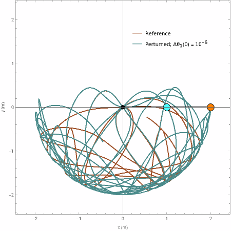
Figure 2: Double-pendulum chaos: solid brown/teal traces start from angles differing by only rad; after a few swings their paths diverge completely, illustrating the sensitive dependence on initial conditions.
-6
10
Example 2 - The N-Body problem
Example 2 - The N-Body problem
The four-body Newtonian system is chaotic: an almost invisible change to one starting velocity can send the future motion onto a completely different path. In the plots shown below, the “reference” panel shows four smooth rosettes traced from perfectly symmetric initial data, while the “perturbed” panel (with just added to one velocity component) quickly departs from that pattern and blooms into a distinct set of loops. Together, the side-by-side orbit plots provide a visual illustration of sensitive dependence on initial conditions, the defining feature of chaotic dynamics in the classical N-body problem.
-6
10
ClearAll["Global`*"];(*parameters*)G=1.;(*gravitationalconstant*)n=4;(*numberofbodies*)m=ConstantArray[1.,n];(*equalmasses*)epsSoft=0.05;(*softeninglength–avoidssingularity*)tmax=40.;(*integrationhorizon*)δv=1.*^-6;(*tinyvelocitytweak*)(*squareofside2aroundtheorigin*)r0={{1.,0.},{-1.,0.},{0.,1.},{0.,-1.}};(*swirl:eachbodygetsatangentialkick*)vMag=0.40;v0={{0.,vMag},{0.,-vMag},{-vMag,0.},{vMag,0.}};(*perturbvxofbody1only*)v0δ=ReplacePart[v0,{1,1}->v0[[1,1]]+δv];(*softenedacceleration*)acc[r_List,i_]:=Sum[-Gm[[j]](r[[i]]-r[[j]])/((Norm[r[[i]]-r[[j]]]^2+epsSoft^2)^(3/2)),{j,DeleteCases[Range[n],i]}];(*integrator*)makeSol[rInit_,vInit_]:=Module[{r=Array[r,n],eq},eq=Flatten@Table[{r[[i]][0]==rInit[[i]],r[[i]]'[0]==vInit[[i]],r[[i]]''[t]==acc[Table[r[[k]][t],{k,n}],i]},{i,n}];NDSolveValue[eq,r,{t,0,tmax},Method->"StiffnessSwitching",MaxStepSize->5.*^-4,AccuracyGoal->12,PrecisionGoal->12]]solRef=makeSol[r0,v0];solPert=makeSol[r0,v0δ];pos[sol_,i_][τ_]:=sol[[i]][τ];
In[]:=
(*colors&linestyles*)col={RGBColor[1,.2,0],RGBColor[.2,.7,0],RGBColor[.2,.4,1],RGBColor[.8,.4,.8]};stylePert=Directive[#,Thick]&/@col;styleRef=Directive[#,Thick,Opacity[.85]]&/@col;curve[i_,sol_,sty_]:=ParametricPlot[Evaluate[sol[[i]][t]],{t,0,tmax},PlotStyle->sty,ColorFunction->None,PlotPoints->900,MaxRecursion->2,PerformanceGoal->"Quality"];refCurves=MapIndexed[curve[#2[[1]],solRef,styleRef[[#2[[1]]]]]&,col];pertCurves=MapIndexed[curve[#2[[1]],solPert,stylePert[[#2[[1]]]]]&,col];startDots=Graphics[Table[{EdgeForm[col[[i]]],FaceForm[col[[i]]],Disk[r0[[i]],0.1]},{i,n}]];legend=LineLegend{Directive[Gray,Thick,Dashed],Directive[Gray,Thick]},"reference","perturbed (Δv₁x = 10⁻⁵)",LegendMarkers->"Line",LabelStyle->13;orbitRefFig=Show[Sequence@@refCurves,startDots,PlotRange->{{-3,3},{-3,3}},AspectRatio->1,Frame->True,PlotLabel->Style["Reference Trajectory \n",14],FrameLabel->(Style[#,13]&/@{"x","y"}),ImageSize->400];orbitPertFig=ShowSequence@@pertCurves,startDots,PlotRange->{{-3,3},{-3,3}},AspectRatio->1,Frame->True,PlotLabel->Style["Perturbed = Trajectory\n",14],FrameLabel->(Style[#,13]&/@{"x","y"}),ImageSize->400;(*finalpresentation*)Grid[{{orbitRefFig,orbitPertFig}}]
x
Δv
1
-6
10
Out[]=
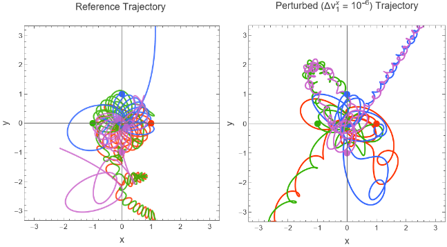
Figure 3: Four-body chaos: a tweak to one body’s initial velocity quickly drives the system away from the reference orbit
-6
10
A bridge to a deeper question
A bridge to a deeper question
Once we acknowledge that the tiniest decimal can dictate a macroscopic fate, an intriguing possibility surfaces: what if a super-intelligence - operating entirely within the laws we know, could “tap” those hidden digits to steer outcomes? Chaos provides the amplifier; the nudge needs only to be small enough to hide beneath measurement noise, yet timed with exquisite accuracy. In the next section, Theological Connections, we will explore how this perspective reinvigorates age-old ideas of providence and cosmic guidance without invoking any suspension of physical law.
Theological Connection: Superior Mind in a Law-Bound Universe
Theological Connection: Superior Mind in a Law-Bound Universe
Many people, across cultures and centuries, have trusted that some higher intelligence or “God” quietly choreographs the unfolding of reality. At the same time, modern science tells a compelling counter-story: everyday events, from an apple falling to a satellite orbiting, obey clear-cut physical laws that engineers test and use with pinpoint accuracy. Seen from that angle, it’s natural to ask:
If the universe already runs on concrete rules that make airplanes fly and smartphones work, where could any guiding super-intelligence still act without breaking those rules?
One clear possible answer lies in deterministic chaos. Chaos theory has taught us that infinitesimal nudges can reshape macroscopic reality. It also affirms that every step of a chaotic system is governed by precise mathematical rules. For philosophers and theologians, this duality - lawful yet unpredictable - opens a fascinating possibility: might a super-intelligence uses chaos to steer the universe without ever breaking its laws?
1. Turning chaos into a steering wheel
1. Turning chaos into a steering wheel
In 1990 Edward Ott, Celso Grebogi, and James A. Yorke (the “OGY” paper, [4]) proved that vanishingly small, well-timed taps can corral a chaotic system onto a desired orbit. Since then, dozens of experimental groups have adapted the “OGY” insight to:
◼
steady semiconductor lasers [5]
◼
nudge cardiac tissue out of fibrillation [6]
◼
damp oscillations on electric-power grids [7]
The required energy is often millions of times smaller than the macroscopic change produced. Thus in principle, a being with perfect knowledge of a system’s micro-state could guide hurricanes, galaxies, or even human history while leaving no obvious fingerprint. This possibility has been explored explicitly by scholars who ask how a super-intelligence might act within, rather than against, the fabric of physics [8-10].

Figure 4: Allegorical portrait of an unseen super-intelligence guiding the cosmic symphony
2. Why daily regularity does not refute chaos (or providence)
2. Why daily regularity does not refute chaos (or providence)
Our coffee still cools according to Newton’s law of cooling, planets orbit per Keplerian ellipses, and photons obey Maxwell’s equations. Chaos does not contradict these laws; it materializes only in nonlinear regimes where feedback loops amplify microscopic uncertainties.
The coexistence of strict laws and wild trajectories suggests that determinism alone does not guarantee human-scale predictability. That gap is precisely the leverage a perfectly informed and minutely economical agent could exploit. A femto-joule puff delivered at the right vortex, a single ion displaced in a neural synapse, is enough to choose one lawful branch of the chaotic tree over another. From our finite perspective nothing looks “miraculous”; the coffee still cools, the photons still diffract, yet a higher intelligence could, in principle, have guided events invisibly through the razor-edge sensitivities that chaos provides.
3. Computational irreducibility: why the “puppeteer” can remain invisible
3. Computational irreducibility: why the “puppeteer” can remain invisible
When you hit [Shift] + [Enter] on a Wolfram notebook that contains a long cellular-automaton evolution, there is no analytic shortcut: Mathematica must grind through every tick, colouring one new row of squares at a time. Stephen Wolfram formalised that stubborn fact as the Principle of Computational Equivalence (PCE) [11]. It states that above a low threshold, simple programs can emulate each other’s complexity, and their outcomes are irreducible: you must run them step-by-step to know what happens.
Suppose, as many physicists now toy with, that the physical universe is a gigantic information-processing machine [12]: space–time cells update via local rules, quantum amplitudes tick like bits. Even if we possessed the complete source code of reality, every field equation, every boundary condition - PCE says we still could not “jump ahead” to tomorrow’s exact weather map, the Dow Jones value, or a photon’s path through a cloud chamber without doing the full calculation.
Thus even an army of physicists - with perfect equations and perfect sensors - would still have to watch the cosmic film frame-by-frame for getting at the outcome. A skilful “puppeteer” who inserts frame-level edits leaves no detectable splice mark; the movie simply unfolds, law-abiding from first scene to last, while its deeper authorship remains forever beyond algorithmic audit.
4. A Wolfram Language glimpse
4. A Wolfram Language glimpse
Here is a conceptual, Wolfram-style blueprint that shows how the layers of consensus physics, chaotic amplification, and microscopic intervention can be nested in one elegant functional expression:
ψ[t+1]=𝒫@𝒞@𝒩[ε(t)]@ψ[t]
ψ[t]
𝒫: Consensus physics operator (Newton, Maxwell, Schrödinger, …)
𝒞: Chaotic mixing operator
𝒩ε: Nudge injector (adds an information pulse)
ε: Infinitesimal control parameter
The regulator sprinkles an attosecond push, chaotic feedback spreads it, and the usual laws carry the now-tilted state forward.
Below is a minimalist toy example that mirrors the idea:
In[]:=
ClearAll[consensusLaws,nudgeInjector,θ,nextState,init,steps,trajNatural,trajGuided,controlStep];(*Consensuslawsforathree-variabletoyuniverse*)consensusLaws={Function[{x,y,z},3.9x(1-x)],(*logisticchaosonx*)Function[{x,y,z},0.99y-0.05z],(*linearcoupling*)Function[{x,y,z},0.05y+0.99z](*energyswap*)};(*controlparameters*)θ=<|"ε"->0.|>;(*Nudgeinjector:usuallyzero,butcanaddεtocoord1*)nudgeInjector={Function[{x,y,z},θ["ε"]],Function[{x,y,z},0],Function[{x,y,z},0]};(*One-stepevolution-chaoticmixingoperatorisasimplePlus*)nextState[s_List]:=MapThread[#1@@s+#2@@s&,{consensusLaws,nudgeInjector}];(*Parameters*)init={0.51,0.2,0.1};steps=150;(*Naturaltrajectory(nonudge)*)trajNatural=NestList[nextState,init,steps];(*Guidedtrajectory:single10⁻⁸tapatstep30*)controlStep=30;trajGuided=FoldList[Function[{state,t},If[t==controlStep,θ["ε"]=10^-8];Module[{new=nextState[state]},θ["ε"]=0;new]],init,Range[steps]];
In[]:=
(*first-coordinatearraysandsmoothing*)
In[]:=
nat1=trajNatural[[All,1]];guid1=trajGuided[[All,1]];smooth[data_]:=GaussianFilter[data,4];natS=smooth[nat1];guidS=smooth[guid1];minLen=Min[Length/@{natS,guidS}];natS=Take[natS,minLen];guidS=Take[guidS,minLen];
(*Theplot*)
In[]:=
colNat=RGBColor["#298cbc"];colGuid=RGBColor["#c46666"];colPulse=GrayLevel[.4];yRange=MinMax[Join[natS,guidS]];xRange={0,minLen-1};ListLinePlot{natS,guidS},
Out[]=
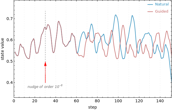
We see that after the injected energy of order at , the two curves are almost the same until about 50th step, after which the guided path peels off dramatically. The nudgeInjector is mathematically legal yet empirically invisible because its parameter θ[“ε”] is virtually always zero. A super-intelligence only needs to toggle θ[“ε”] at opportune instants to reroute the future.
-8
10
step=30
Scale this example to degrees of freedom and the moral remains unchanged - the super-intelligence has all the steering room it needs without ever editing the visible laws.
100
10
5. Science writes models, not mandates
5. Science writes models, not mandates
Finally, it is important to note that we hold only models which are compact stories that summarize everything we have measured so far (even if it is trillion number of time). We measure, then generalize and predict; the reality either cooperates or sends us back to the chalkboard. In that sense the cosmos is not obeying our formulas; we are describing its habits, always tentatively and always subject to revision. Here are some notable examples:
◼
Newton’s 𝐹 = 𝑚 𝑎 ruled mechanics for two centuries until Einstein showed that at relativistic speeds the relation warps into = 𝑚 inside curved space-time. [13]
𝜇
𝐹
𝜇
a
◼
Paul Dirac and, later, John Barrow wondered whether “constants” like 𝐺 (Newton’s gravitational constant) or 𝛼 (fine-structure constant) might drift over cosmic time. Even a one-in-a-million shift would rewrite the periodic table and expose how provisional our “laws” really are. [14-15]
So, yes: in a logically possible tomorrow the apple might accelerate at twice the rate predicted by today’s . Our equations would not “break”; they would simply stop fitting the data, and have to scramble for a deeper model.
F=ma
Thus since the modeled or formulated laws are at best the current best fit, their very changeability keeps open the logical space for higher-order control. A super-intelligence could revise them, or let them mutate, without consulting our textbooks. Deterministic chaos would merely amplify the consequence.
References
References
1. Strogatz, S. H. (2024). Nonlinear dynamics and chaos: with applications to physics, biology, chemistry, and engineering. Chapman and Hall/CRC.
2. Devaney, R. (2018). An introduction to chaotic dynamical systems. CRC press.
3. Alligood, K. T., Sauer, T. D., & Yorke, J. A. (1997). Chaos: an introduction to dynamical systems. New York, NY: Springer New York.
4. Ott, E., Grebogi, C., & Yorke, J. A. (1990). Controlling chaos. Physical review letters, 64(11), 1196.
5. Bielawski, S., Derozier, D., & Glorieux, P. (1994). Controlling unstable periodic orbits by a delayed continuous feedback. Physical Review E, 49(2), R971.
6. Garfinkel, A., Spano, M. L., Ditto, W. L., & Weiss, J. N. (1992). Controlling cardiac chaos. Science, 257(5074), 1230-1235.
7. Dorfler, F., & Bullo, F. (2012). Synchronization and transient stability in power networks and nonuniform Kuramoto oscillators. SIAM Journal on Control and Optimization, 50(3), 1616-1642.
8. Polkinghorne, J. C. (2009). Science and providence: God’s interaction with the world. Templeton Foundation Press.
9. Russell, R. J., Murphy, N., & Peacocke, A. R. (1995). Chaos and Complexity: Scientific Perspectives on Divine Action Vatican Observatory and Berkeley: CTNS.
10. Murphy, N. C., & Ellis, G. F. R. (1996). On the moral nature of the universe: Theology, cosmology, and ethics (Vol. 137). Fortress Press.
11. Wolfram, S. (1997). New kind of science.
12. t Hooft, G. (2016). The cellular automaton interpretation of quantum mechanics (p. 298). Springer Nature.
13. C. W. Misner, K. S. Thorne & J. A. Wheeler (1973), Gravitation. W. H. Freeman.
14. Dirac, P. A. (1937). The cosmological constants. Nature, 139(3512), 323-323.
15. Barrow, J. (2005). Varying constants. Philosophical Transactions of the Royal Society A: Mathematical, Physical and Engineering Sciences, 363(1834), 2139-2153.
CITE THIS NOTEBOOK
CITE THIS NOTEBOOK
From decimal dust to divine design: precision, chaos, and the question of cosmic control
by Jayanta Phadikar
Wolfram Community, STAFF PICKS, July 14, 2025
https://community.wolfram.com/groups/-/m/t/3511154
by Jayanta Phadikar
Wolfram Community, STAFF PICKS, July 14, 2025
https://community.wolfram.com/groups/-/m/t/3511154