This project focuses on addressing the essential question: “To what extend does varying the complexity of neural networks affect their efficiency in learning mathematical functions, and how can these changes be quantitatively measured?” The intent is to investigate the relationship between the complexity of neural networks and their capability to learn mathematical functions, while simultaneously creating an effective methodology for quantitative assessment of these variations.
Keywords:
Keywords:
Neural Networks: a model built with interconnected nodes (or neurons), which work together to process information. Neural Networks learn from input data by adjusting strengths of these connections.
Activation function: a mathematical calculation that introduces non-linearity into the network’s learning process, enables the network to learn complex data.
Loss: refers to a function that calculates the difference between the model’s prediction and the actual input from the given data. Represents the precision of the neural network in learning the inputs
Defining the first criteria to analyze complexity: The amount of neurons in a neural network
Defining the first criteria to analyze complexity: The amount of neurons in a neural network
Objective in this section: to obtain the appropriate domain of numbers of neurons that could be applied to the neural network model
Model for training - Varying the number of neurons:
Model for training - Varying the number of neurons:
Choosing one function to generate data for training
In[]:=
Exp[-Norm[{x,y}]]//NormalmultiNeuronData=Flatten@Table[{x,y}->Exp[-Norm[{x,y}]],{x,-3,3,.005},{y,-3,3,.005}];Short[multiNeuronData,2]
Out[]=
-+
2
Abs[x]
2
Abs[y]
Out[]//Short=
{{-3.,-3.}0.0143696,{-3.,-2.995}0.0144205,1442398,{3.,3.}0.0143696}
Here, a list of training data is being generated from the function Exp[-Norm[{x,y}]] in the given range [-3,x,3], [-3,y,3].
These data are then being applied to neural networks with different numbers of neurons
These data are then being applied to neural networks with different numbers of neurons
Varying complexities of neural network by changing the number of neurons, n as the variable:
net=NetChain[{2^n,Tanh,1}]
The amount of neurons in the neural network will increment by a factor of 2 every time the network is trained.
An example of training a neural network, using 2^5, 32 neurons, in 3 layers:
net=NetChain[{32,Tanh,1}];multiNeuroTrained=NetTrain[net,multiNeuronData,All,MaxTrainingRounds2,ValidationSetScaled[0.2]]
Out[]=
NetTrainResultsObject
There are many properties of a neural net that could generate useful data to analyze Efficiency vs Complexity (For example, TotalTrainingTime), however, we will only be extracting the final average loss among all these properties to compare the performance.
Training Data with different amount of neurons:
Training Data with different amount of neurons:
Generating training data, and RoundLossList across 2^0 - 2^10 numbers of neurons.
The purpose of this section is to generate enough data for a primary analysis on the proper domain that the training should be limited to. Neural networks with certain complexities that fail to provide a proper learning precision would be excluded from future trainings.
The purpose of this section is to generate enough data for a primary analysis on the proper domain that the training should be limited to. Neural networks with certain complexities that fail to provide a proper learning precision would be excluded from future trainings.
Properties with 1(2^0) starting neuron
Properties with 1(2^0) starting neuron
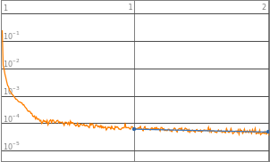
Initializing the net, graphing the LossPlot, and extracting the RoundLossList
net=NetChain[{1,Tanh,1}];trained1=NetTrain[net,data,All,MaxTrainingRounds2,ValidationSetScaled[0.2]];
In[]:=
(*Neurons:1*)trained1["LossPlot"]
Out[]=

In[]:=
trained1["RoundLossList"]
Out[]=
{0.0214701,0.0213977}
Properties with 2(2^1) starting neurons
Properties with 2(2^1) starting neurons
Properties with 4(2^2) starting neurons
Properties with 4(2^2) starting neurons
Properties with 8(2^3) starting neurons
Properties with 8(2^3) starting neurons
Properties with 16(2^4) starting neurons
Properties with 16(2^4) starting neurons
Properties with 32(2^5) starting neurons
Properties with 32(2^5) starting neurons
Properties with 64(2^6) starting neurons
Properties with 64(2^6) starting neurons
Properties with 128(2^7) starting neurons
Properties with 128(2^7) starting neurons
Properties with 256(2^8) starting neurons
Properties with 256(2^8) starting neurons
Properties with 512(2^9) starting neurons
Properties with 512(2^9) starting neurons
Properties with 1024(2^10) starting neurons
Properties with 1024(2^10) starting neurons
Visualization:
Visualization:
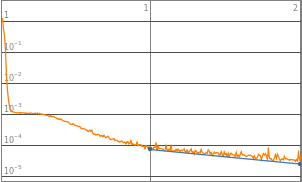
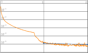
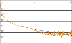
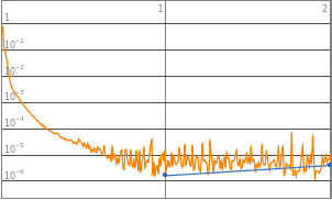
Aligning the LossPlots, along with level of complexities to visualize the accuracy of learning model
In[]:=
Grid[Table[{Style[StringJoin["2^",ToString[n],"(",ToString[2^n],")"],20],Symbol[StringJoin["trained",ToString[2^n]]]["LossPlot"]},{n,0,10}],Frame->All,Spacings->2]
Out[]=
2^0(1) | |||
2^1(2) | |||
2^2(4) | |||
2^3(8) | |||
2^4(16) | |||
2^5(32) | |||
2^6(64) | |||
2^7(128) | |||
2^8(256) | |||
2^9(512) | |||
2^10(1024) |
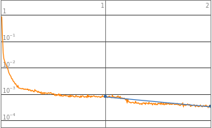
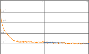

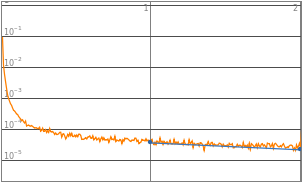
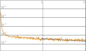
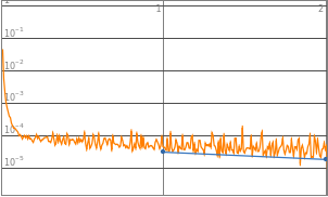
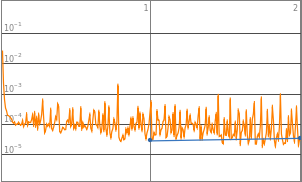
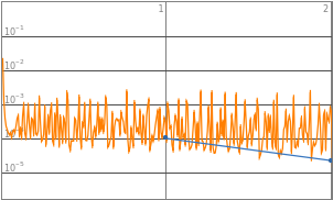
By observing the data, neural networks with 2^0 to 2^3 starting neurons appears to be insufficient enough to train the neural network, they are the “outliers” data points that are not helpful in finding the optimized complexity for best performance. Therefore, properties of 2^0 to 2^3 will be eliminated in the following analysis. Vice versa, neural network with 2^10 neurons displays a significant amount of noises thus 2^10 will also be excluded from future training.
Conclusion:
Conclusion:
Puling out a list of the final average loss of each function.
In[]:=
lossData=Table[{n,Symbol[StringJoin["trained",ToString[2^n]]]["RoundLossList"][[2]]},{n,4,9}]
Out[]=
{{4,0.000119835},{5,0.0000591963},{6,0.0000345127},{7,0.0000331252},{8,0.000050523},{9,0.000119795}}
Graphing the LossList across different numbers of neurons
ListLinePlotlossData,
Out[]=
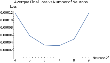
The graph of final average loss vs 2^n numbers of neurons provide a direct visualization of a function roughly the shape of a parabola. With this graph, we can conclude that neither too little or too much neurons in a neural network would improve the accuracy; as well, the parabolic shape indicates that there will be an “optimized” amount of neurons in a neural network that would provide the highest precision, which could be a representation of the complexity of the math function
Defining the second criteria to analyze complexity: The number of layers
Defining the second criteria to analyze complexity: The number of layers
Objective in this section: to obtain the appropriate domain of numbers of layers that could be applied to the neural network model
Model for training - Varying the number of layers:
Model for training - Varying the number of layers:
Choosing one function to generate data for training
In[]:=
-Log[x^2+1]//NormalmultiLayerData=Flatten@Table[{x,y}->x,{x,-3,3,.005},{y,-3,3,.005}];Short[multiNeuronData,2]
Out[]=
-Log[1+]
2
x
Out[]//Short=
{{-3.,-3.}0.0143696,{-3.,-2.995}0.0144205,1442398,{3.,3.}0.0143696}
A list of training data is being generated from the function -Log[x^2+1] in the given range [-3,x,3], [-3,y,3].
These data are then being applied to neural networks with different number of layers
These data are then being applied to neural networks with different number of layers
Here, we are training an example neural network that has 5 layers in total, with 3 linear layers having 8 neurons each.
However, even though the number of layers varies, the order of the layers follows a pattern: a linear layer with multiple neurons + activation function tanh + n linear layers with multiple neurons + a linear layer with one neuron.
However, even though the number of layers varies, the order of the layers follows a pattern: a linear layer with multiple neurons + activation function tanh + n linear layers with multiple neurons + a linear layer with one neuron.
In[]:=
multiLayerModel=NetChain[Insert[Flatten[{Table[LinearLayer[8],{x,1,3}],LinearLayer[1]}],ElementwiseLayer[Tanh],2]]
Out[]=
NetChain

multiLayerTrained=NetTrain[multiLayerModel,multiLayerData,All,MaxTrainingRounds2,ValidationSetScaled[0.2]]
Out[]=
NetTrainResultsObject

Pulling out the data from the example multilayer network
In[]:=
MultiLayerTrained["LossPlot"]
Out[]=
In[]:=
MultiLayerTrained["RoundLossList"]
Out[]=
{0.0163135,0.0000561487}
Training Data with different amount of layers:
Training Data with different amount of layers:
This subsection is intended to generate enough data for a primary analysis on the proper domain that the training should be limited to regarding the number of layers. Neural networks that produce high precision will be kept, networks that produces insufficient precision would be excluded from future trainings.
Properties with 3 layers
Properties with 3 layers
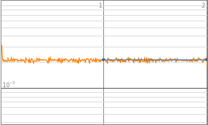
Initializing the net, graphing the LossPlot, and extracting the RoundLossList
layerModel1=NetChain[Insert[Flatten[{Table[LinearLayer[8],{x,1,1}],LinearLayer[1]}],ElementwiseLayer[Tanh],2]];layerTrained1=NetTrain[layerModel1,multiLayerData,All,MaxTrainingRounds2,ValidationSetScaled[0.2]];
In[]:=
layerTrained1["LossPlot"]
Out[]=
In[]:=
layerTrained1["RoundLossList"]
Out[]=
{0.00650892,9.21766×}
-6
10
Properties with 4 layers
Properties with 4 layers
Properties with 5 layers
Properties with 5 layers
Properties with 6 layers
Properties with 6 layers
Properties with 7 layers
Properties with 7 layers
Properties with 8 layers
Properties with 8 layers
Visualization:
Visualization:
Aligning the LossPlots, along with level of complexities to visualize the accuracy of learning model
In[]:=
Grid[Table[{Style[StringJoin[ToString[n+2]," layers"],20],Symbol[StringJoin["layerTrained",ToString[n]]]["LossPlot"]},{n,1,6}],Frame->All,Spacings->2]
Out[]=
3 layers | |||
4 layers | |||
5 layers | |||
6 layers | |||
7 layers | |||
8 layers |

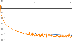
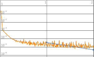
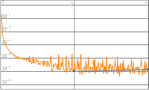
Neural networks with 3 to 8 layers all produced a decent loss. Therefore the domain of layers would be set to 3-8 layers, such that it could accommodate a wider range of functions input.
Conclusion:
Conclusion:
Puling out a list of the final average loss of each function:
In[]:=
layerData=Table[{n+2,Symbol[StringJoin["layerTrained",ToString[n]]]["RoundLossList"][[2]]},{n,1,6}]
Out[]=
{{3,9.21766×},{4,7.84575×},{5,7.51481×},{6,0.0000120899},{7,0.000018011},{8,0.0000250827}}
-6
10
-6
10
-6
10
Graphing the LossList across different numbers of layers:
ListLinePlotlayerData,
Out[]=
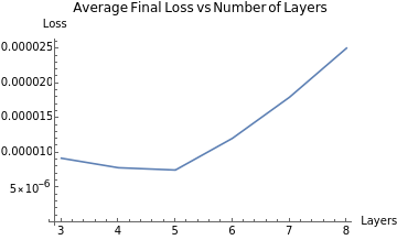
The graph of final average loss vs n number of layers also displays a function roughly the shape of a parabola. With this graph, we can make similar conclusion that we got from the neurons chapter: neither too little or too much layers in a neural network would improve the accuracy; as well, there will be an "optimized" amount of layers in a neural network that would provide the highest precision, which could be a representation of the complexity of the math function.
Abstracting Algorithm
Abstracting Algorithm
Objective in this section: to abstract previous code & to make one function that could iterate through all neural network and output the most optimized points
Generating Data:
Generating Data:
Making one function that takes in a math formula and generate a list of data
generateData[func_]:= Flatten@Table[{x,y}->func,{x,-3,3,.01},{y,-3,3,.01}];
Training a single Neural Net:
Training a single Neural Net:
Making a function that takes in data, number of neurons, number of layers, and train a network according to inputted parameters
trainSingleNet[data_,complexity_, layer_] := Module[{net, trainedNet},net = NetChain[Insert[Flatten[{Table[LinearLayer[complexity],{x,1,layer}], LinearLayer[1]}],ElementwiseLayer[Tanh],2]];trainedNet = NetTrain[net,data,All,MaxTrainingRounds->8,ValidationSetScaled[0.2]];trainedNet]
Looping through all neuron complexities:
Looping through all neuron complexities:
Making a function that would iterate through all number of neurons in the set domain, outputs a list of loss data.
In[]:=
trainNeurons[func_,layer_,data_]:=Module[{lossData, neuMin = 4, neuMax = 9},Table[trainedNet[2^n] = trainSingleNet[data, 2^n, layer],{n,neuMin,neuMax}];lossData = Table[{n,layer, trainedNet[2^n]["RoundLossList"][[8]]}, {n,neuMin,neuMax}];lossData]
Looping through layers:
Looping through layers:
Making a function that would iterate through all the layers in the set domain, outputs a compiled list of loss data
In[]:=
trainLayers[func_,data_]:=Module[{list3D, layMin=1, layMax=6},list3D = Flatten[Table[trainNeurons[func, n, data],{n, layMin, layMax}],1];list3D]
Putting everything together:
Putting everything together:
How it works
How it works
Pulling an example of compiled list of loss data.
networkInfoList=trainLayers[x]
Out[]=
{{4,1,0.00145321},{5,1,0.000221956},{6,1,0.000312871},{7,1,0.0000704327},{8,1,0.0000788333},{9,1,0.000179943},{4,2,0.000129808},{5,2,0.0000879509},{6,2,0.000123718},{7,2,0.000427584},{8,2,0.000713873},{9,2,0.000891467},{4,3,0.0000766274},{5,3,0.000125055},{6,3,0.00022729},{7,3,0.000411139},{8,3,0.000671742},{9,3,0.00111959},{4,4,0.00008248},{5,4,0.000164488},{6,4,0.000283265},{7,4,0.000553571},{8,4,0.00657161},{9,4,0.57834},{4,5,0.000152367},{5,5,0.000210252},{6,5,0.000388681},{7,5,0.000646598},{8,5,0.0729928},{9,5,14.7071},{4,6,0.000171376},{5,6,0.000285941},{6,6,0.00044167},{7,6,0.00065832},{8,6,0.558543},{9,6,33328.1}}
Visualizing the loss data from different complexity on a 3D model
In[]:=
networkPlot=ListPlot3D[{networkInfoList},AxesLabel{"Number of Neurons(2^n)","Number of Layers(n)","Loss"}]
Out[]=

Calculating the optimized point according to the lowest loss
In[]:=
opPoint=TakeSmallestBy[l,Last,1]
Out[]=
{{7,1,0.0000704327}}
The opPoint is constructed by {number of neurons 2^n, number of layers n, loss}. This data structure allows accessible comparison across multiple functions.
Abstraction
Abstraction
Abstracting all the functions into one function
In[]:=
trainNeuralNet[func_]:=Module[{opPoint,data},data = generateData[func];opPoint = Flatten[{TakeSmallestBy[trainLayers[func,data],Last,1], func}];opPoint]
By calling trainNeuralNet function, all the abstracted functions would be called, with the most optimized point in the format {neurons, layers, loss, function} being returned.
Analysis
Analysis
Defining the Evaluation matrix
Defining the Evaluation matrix
We are creating an evaluation matrix to plot the most optimized neural net for math functions, while looking for patterns in the points plotted
The matrix has 2 axis, its x-axis being the number of neurons, and its y-axis being the number of layers.
The matrix has 2 axis, its x-axis being the number of neurons, and its y-axis being the number of layers.
Setting the domain and range of the evaluation matrix:
ListPlot{{4,1},{9,6}},
Out[]=
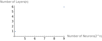
The domain of the number of neurons includes 2^4 to 2^9 neurons, the range of the layers includes 1 to 6 layers in addition to 1 Tanh activation layer and 1 linear layer. The evaluation matrix displays neural networks of different complexity.
An example {4,3} means that the neural network has 2^4 16 neurons and 3+2 5 layers.
An example {4,3} means that the neural network has 2^4 16 neurons and 3+2 5 layers.
Optimized neural net complexity with different group of math functions
Optimized neural net complexity with different group of math functions
Calculating the most optimized net for some example math functions, these functions cover a wide range of mathematical operation, with varied coefficients.
Trigonometric functions
Trigonometric functions
Calling trainNeuralNet with trig functions
In[]:=
trigSin=trainNeuralNet[Sin[x]]
Out[]=
{4,3,0.000156019,Sin[x]}
In[]:=
trig3Sin=trainNeuralNet[3Sin[x]]
Out[]=
{4,3,0.000853865,3Sin[x]}
Polynomials
Polynomials
Calling trainNeuralNet with polynomials functions
In[]:=
polyx2=trainNeuralNet[x^2]
Out[]=
{5,2,0.00175294,}
2
x
In[]:=
poly12x2=trainNeuralNet[12x^2]
Out[]=
{4,3,0.134422,12}
2
x
Logarithmic functions
Logarithmic functions
Calling trainNeuralNet with Log functions
In[]:=
log10=trainNeuralNet[Log[10,(x^2)+1]]
Out[]=
7,1,0.000018131,
Log[1+]
2
x
Log[10]
In[]:=
log2=trainNeuralNet[Log[2,(x^2)+1]]
Out[]=
7,1,0.0000551542,
Log[1+]
2
x
Log[2]
Exponential functions
Exponential functions
Calling trainNeuralNet with exponents functions
In[]:=
exp2x=trainNeuralNet[2^x]
Out[]=
{8,1,0.00140252,}
x
2
expSinx=trainNeuralNet[E^Sin[x]]
Out[]=
8,1,0.000312915,
Sin[x]
Observing patterns from the data
Observing patterns from the data
Plotting out the data points on the evaluation matrix
ListPlot{Labeled[Take[trigSin,2],trigSin[[4]],Right],Labeled[Take[trig3Sin,2],trig3Sin[[4]],Right],Labeled[Take[polyx,2],polyx[[4]],Right],Labeled[Take[polyx2,2],polyx2[[4]],Right],Labeled[Take[poly12x2,2],poly12x2[[4]],Right],Labeled[Take[log10,2],log10[[4]],Right],Labeled[Take[exp2x,2],exp2x[[4]],Right],Labeled[Take[expSinx,2],expSinx[[4]],Right]},
Out[]=
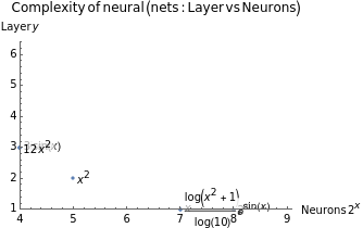
There are a few neural net complexities {neurons, layers} where the optimized point of math function clusters: {4,3}, {7,1}, {8,1}
But how are they related to how the neural net learn and adapt to each mathematical function? We will graph the activation function Tanh[x], as well as the functions that have similar optimized neural net complexities.
But how are they related to how the neural net learn and adapt to each mathematical function? We will graph the activation function Tanh[x], as well as the functions that have similar optimized neural net complexities.
Neural net cluster at {4,3}
Neural net cluster at {4,3}
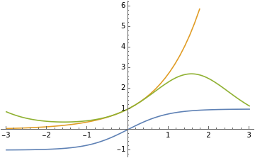
Plotting the functions that clusters around {4,3}
In[]:=
Plot[{Tanh[x],Sin[x],3Sin[x],12x^2},{x,-3,3},PlotLegends->"Expressions"]
Out[]=
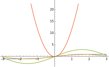
Functions that cluster at {4,3} doesn’t change concavity, or if any, concavity is only changed at 0. Coefficient also has no effect on how a neural network learns, as sin[x] and 3sin[x] share the same optimized net.
Neural net cluster at {7,1}
Neural net cluster at {7,1}
Plotting the functions that clusters around {7, 1}
In[]:=
Plot[{Tanh[x],Log[10,(x^2)+1],Log[2,(x^2)+1]},{x,-3,3},PlotLegends->"Expressions"]
Out[]=
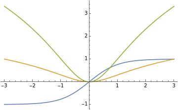
Functions that cluster at {7,1} changes concavity more than twice in the domain {x,-3,3}.
Neural net cluster at {8,1}
Neural net cluster at {8,1}
Plotting the functions that clusters around {8,1}
In[]:=
Plot[{Tanh[x],E^x,E^Sin[x]},{x,-3,3},PlotLegends->"Expressions"]
Out[]=
Functions that cluster at {8, 1} have no intersection with Tanh[x] in the domain[x,-3,3], more adjustments are required be made for Tanh[x] in order to model these functions.
Result:
Result:
The complexity variation of neural networks are dependent on the shape of math functions, independent on the coefficient and the scale of the function .
Conclusion:
Conclusion:
Summary:
Summary:
In conclusion, we’ve developed a new approach to understand the complexity of a mathematical function, by uniquely representing each math function with an optimized neural network. We’ve established a correlation between the number of neurons, number of layers of a neural network, and the complexity of mathematical functions; and created an evaluation matrix, which stands as a helpful tool to quantitatively measure the complexity of a mathematical function.
Limitations:
Limitations:
◼
The activation function is for all trained neural network is Tanh, parabolic tangent function
◼
The function needs to be defined over the entire domain, otherwise there might be error, as the structure of the training data is constructed as {x,y} -> value
◼
The neuron and layer values are limited to integers.
◼
The neural network learning models were only trained for 2 rounds
Future Works:
Future Works:
◼
To relate the mathematical principles of backpropagation with the patterns that are displayed between mathematical functions and complexities of optimized neural net models
◼
Interpolate data points into mathematical functions, then use the functions to find more precise value for optimization points.
◼
Run the algorithm with more mathematical functions, obtain the optimized points and plot them into the evaluation matrix, for a more accurate, intuitive graph.
◼
Run the algorithm with different activation functions to observe change in the output.
Acknowledgements:
Acknowledgements:
I wish to express my deepest gratitude to my mentor Eric Rimbey, who provided me insightful guidance and constructive criticisms throughout the research.
Special thanks to Nicolo Monti for his valuable suggestions during this project, and to Wolfram Summer Research Program for providing me this opportunity to explore in the field of machine learning.
Special thanks to Nicolo Monti for his valuable suggestions during this project, and to Wolfram Summer Research Program for providing me this opportunity to explore in the field of machine learning.
Citations:
Citations:
“What Is Chatgpt Doing ... and Why Does It Work?” Stephen Wolfram Writings RSS, 14 Feb. 2023,
https://writings.stephenwolfram.com/2023/02/what-is-chatgpt-doing-and-why-does-it-work/ .
https://writings.stephenwolfram.com/2023/02/what-is-chatgpt-doing-and-why-does-it-work/ .
Wolfram Language & amp; System Documentation Center,
https://reference.wolfram.com/language/ . Accessed 12 July 2023. z
https://reference.wolfram.com/language/ . Accessed 12 July 2023. z
CITE THIS NOTEBOOK
CITE THIS NOTEBOOK
Evaluating the impact of complexity variation in neural nets on learning Math functions
by Tianyu Shen
Wolfram Community, STAFF PICKS, July 13, 2023
https://community.wolfram.com/groups/-/m/t/2963315
by Tianyu Shen
Wolfram Community, STAFF PICKS, July 13, 2023
https://community.wolfram.com/groups/-/m/t/2963315