The Wolfram Emerging Leaders Program: High School (WELP:HS) is a remote, semester-long program designed for exceptional graduates from the Wolfram High School Summer Research Program to continue to develop their skills. Students work in a small group over the course of a semester to do either a research-based project or a product development–based project under the guidance of expert mentors. Projects are centered around a topic at the intersection of the group’s interests.
This essay was written by:
This project looks to explore a new kind of hash function for more secure encryption via the chaotic motion of a double pendulum, for use in post-quantum applications. We simulate a double pendulum and solve for the equations of motions symbolically to determine how various input parameters and initial conditions affect the output for hashing. To compare the results of our hash function, we compared the effectiveness of the function with other common functions, such as MD5 and SHA-256, with metrics like Hamming distance and bit uniformity.
Introduction
Introduction
Currently, one of the most popular forms of secure information technology is RSA (Rivest-Shamir-Adleman), which is based on the difficulty of factoring large integers. As the integers get linearly bigger, the factorizations become exponentially more difficult. However, quantum computers have heightened capabilities in factorizing numbers compared to classical computers thanks to Shor’s algorithm, which means eventually quantum computing will reach a point where it could break RSA and other similar forms of encryption, such as elliptic-curve cryptography. As a result, development is currently being made in the field of Post-Quantum Cryptography (PQC), with ideas such as finding the best vector basis for a set of points. In this paper, we explore an alternative PQC algorithm for encryption, which employs the chaotic behavior of a double pendulum. By tweaking and choosing specific input parameters to track, we can solve for motion-based parameters and use that to create a hash function for strings.
Chaotic Behavior and Double Pendulums
Chaotic Behavior and Double Pendulums
Chaotic behavior refers to the unpredictable, yet deterministic, evolution of systems governed by nonlinear dynamics. In chaotic systems, such as the double pendulum, small changes in initial conditions lead to vastly divergent outcomes, a phenomenon known as sensitivity to initial conditions. This sensitivity makes chaotic systems highly sensitive to minor variations in input, resulting in outcomes that appear random despite being governed by precise mathematical rules. The double pendulum, with its two arms swinging in an interdependent motion, serves as a striking example of this behavior, where slight adjustments in angle or velocity can result in dramatically different trajectories over time. This inherent unpredictability and complexity are central to chaos theory, which explores how systems that seem random on the surface can still follow deterministic laws. The sensitivity of chaotic systems to initial conditions makes them ideal for generating random outcomes, offering a powerful tool for simulations, cryptography, and modeling complex phenomena where small changes can have large, unforeseen impacts. Here, we leverage the randomness that the double pendulum creates for use in a cryptographic setting, namely a hash function.
Creating the Double Pendulum (DP) Simulation
Creating the Double Pendulum (DP) Simulation
The approach we used to create the Double Pendulum simulation takes advantage of one of the Wolfram Language’s key strengths: its ability to solve systems of equations symbolically. By formulating the system with symbols and parameters, we can generate exact solutions that represent the physical motion of the double pendulum. This involves defining variables like angles, angular velocities, and masses, and then deriving the equations of motion through Newtonian mechanics.
Variables and their Meanings
Variables and their Meanings
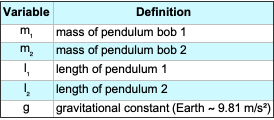
Here, we define and describe the variables used in the chaotic double pendulum model. These variables represent the physical parameters that influence the system’s motion and ultimately contribute to the hash function’s chaotic behavior.
Out[]=
Derive the Equations of Motion using Newton’s 2nd Law
Derive the Equations of Motion using Newton’s 2nd Law
These equations represent the application of Newton’s Second Law to the double pendulum system. The forces acting on each mass in the x and y directions are summed to determine their respective accelerations. The transition from the visual representation of the system to these equations involves resolving the forces due to gravity and tension in the rods, which will be further broken down in the derivation process.


In[]:=
deqns={Subscript[m,1]x1''[t]==(λ1[t]/Subscript[l,1])x1[t]-(λ2[t]/Subscript[l,2])(x2[t]-x1[t]),Subscript[m,1]y1''[t]==(λ1[t]/Subscript[l,1])y1[t]-(λ2[t]/Subscript[l,2])(y2[t]-y1[t])-Subscript[m,1]g,Subscript[m,2]x2''[t]==(λ2[t]/Subscript[l,2])(x2[t]-x1[t]),Subscript[m,2]y2''[t]==(λ2[t]/Subscript[l,2])(y2[t]-y1[t])-Subscript[m,2]g}
Out[]=
[t]-,[t]-g+-,[t],[t]-g+
m
1
′′
x1
x1[t]λ1[t]
l
1
(-x1[t]+x2[t])λ2[t]
l
2
m
1
′′
y1
m
1
y1[t]λ1[t]
l
1
(-y1[t]+y2[t])λ2[t]
l
2
m
2
′′
x2
(-x1[t]+x2[t])λ2[t]
l
2
m
2
′′
y2
m
2
(-y1[t]+y2[t])λ2[t]
l
2
The variable is named “deqns” as a shorthand for “differential equations,” which accurately describes its role in the code. These equations govern the motion of the double pendulum by defining the second-order differential relationships between the system’s masses, lengths, and forces. Since the equations explicitly describe how acceleration is determined by forces acting on each pendulum bob, using a name that reflects this mathematical structure is appropriate.
Represent Algebraic Constants
Represent Algebraic Constants
The lengths of the rods, and , are fixed and can be represented in terms of their 𝑥[𝑡] and 𝑦[𝑡] coordinates. Since the pendulum bobs move in a constrained motion, their positions must satisfy these algebraic equations at all times. These constraints ensure that the distances between the pendulum bobs remain constant, maintaining the physical structure of the system.
l
1
l
2
In[]:=
aeqns={x1[t]^2+y1[t]^2==Subscript[l,1]^2,(x2[t]-x1[t])^2+(y2[t]-y1[t])^2==Subscript[l,2]^2}
Out[]=
{+,+}
2
x1[t]
2
y1[t]
2
l
1
2
(-x1[t]+x2[t])
2
(-y1[t]+y2[t])
2
l
2
The variable is named “aeqns” as a shorthand for “algebraic equations.” These equations define the constraints that enforce the fixed lengths of the rods, ensuring that the double pendulum follows a physically accurate motion.
Specify the Initial State of the System
Specify the Initial State of the System
This is where the symbolic computation of the Wolfram Language is put to use as we define the initial conditions of the simulation as symbolic constants. These represent the initial coordinates of both pendulums.
In[]:=
ics={x1[0]==1,y1[0]==0,y1'[0]==0,x2[0]==1,y2[0]==-1,y2'[0]==0};
Specify Physical Parameters
Specify Physical Parameters
Additionally, we use symbolic constants to specify the initial state of the Double Pendulum System.
In[]:=
params={g->9.81,Subscript[m,1]->1,Subscript[m,2]->1,Subscript[l,1]->1,Subscript[l,2]->1}
Out[]=
{g9.81,1,1,1,1}
m
1
m
2
l
1
l
2
Solve and Visualize the System
Solve and Visualize the System
Here, we are solving the system of differential equations governing the motion of the double pendulum using NDSolve. This function is used to numerically approximate solutions to differential equations, which is necessary given the complexity and chaotic nature of the system. The Method option is set to {“IndexReduction” -> {“Pantelides”, “ConstraintMethod” -> “Projection”}} to handle the algebraic constraints imposed by the fixed rod lengths. These constraints ensure that the pendulum bobs remain at a fixed distance from their pivot points, preventing numerical drift that could introduce unrealistic motion.
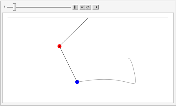
After solving for the positions of the pendulum bobs over time, we visualize the system using an animation. The red and blue dots represent the two masses, and their trajectories trace out the chaotic motion of the double pendulum. The Animate function continuously updates the positions of the masses and the connecting rods, while a gray line shows the historical path of the second pendulum bob. This visualization helps illustrate the unpredictable nature of the motion, which is a key component in making this system useful for chaotic hashing.
In[]:=
soldp=First[NDSolve[{deqns,aeqns,ics}/.params,{x1,y1,x2,y2,λ1,λ2},{t,0,15},Method->{"IndexReduction"->{"Pantelides","ConstraintMethod"->"Projection"}}]];Animate[Graphics[{{PointSize[.025],{Red,Point[{x1[t],y1[t]}]},{Blue,Point[{x2[t],y2[t]}]},Line[{{0,0},{x1[t],y1[t]},{x2[t],y2[t]}}]}/.soldp,{Gray,Line[Map[Function[Evaluate[{x2[#],y2[#]}/.soldp]],Range[0,t,0.025]]]}},PlotRange->{{-2,2},{-2,0}},Axes->True,Ticks->False,ImageSize->500],{t,0,10,.025},SaveDefinitions->True]
Out[]=
Optimizing Randomness Parameters
Optimizing Randomness Parameters
With the simulation of the Double Pendulum system complete, we now have a list of parameters different configurations of which can generate widely different results, a key feature of chaotic systems. The next task is to find the configurations which generate the most randomness. Later, this will prove invaluable in generating random hashes for adjacent input strings.
Plotting Randomness of Variable Across Time steps
Plotting Randomness of Variable Across Time steps
In order to create the environment to test different configurations of input parameters, we need to be able to plot changes in one parameter at a time, shown below.
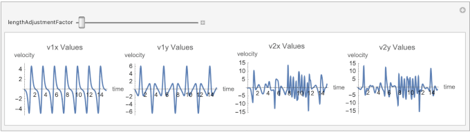
The parameter lengthAdjustmentFactor represents an incremental adjustment to the lengths of the pendulum rods and ).
(
l
1
l
2
The modifierRange variable determines the range of values that the parameter lengthAdjustmentFactor can take in the interactive simulation. This range influences the system by modifying the pendulum lengths ( and ), which in turn affects the chaotic motion of the double pendulum. By varying lengthAdjustmentFactor, we can explore how small changes in initial conditions lead to different trajectories, highlighting the system’s sensitivity to initial parameters.
(
l
1
l
2
The randomness in the system can be observed in the velocity plots for different values of lengthAdjustmentFactor. As the length changes, the system exhibits varying degrees of unpredictability, which is evident in the fluctuations of v1x, v1y, v2x, and v2y. For larger values of lengthAdjustmentFactor, the system becomes increasingly chaotic, with more drastic changes in velocity, demonstrating how small perturbations lead to diverging behaviors over time.
In[]:=
tValues=Range[0,15,0.01];modifierRange={1,10};lengthManipulate=Quiet@Manipulate[Module[{params,ics,soldp,v1x,v1y,v2x,v2y,v1xValues,v1yValues,v2xValues,v2yValues},(*Updatelengthandinitialconditions*)params={g->9.81,Subscript[m,1]->1,Subscript[m,2]->1,Subscript[l,1]->1,Subscript[l,2]->lengthAdjustmentFactor};ics={x1[0]==1+0.1*lengthAdjustmentFactor,x1'[0]==0,y1[0]==0,y1'[0]==0,x2[0]==1,x2'[0]==0,y2[0]==-1,y2'[0]==0};soldp=First[Quiet[NDSolve[{deqns,aeqns,ics}/.params,{x1,y1,x2,y2,λ1,λ2},{t,0,15},Method->{"IndexReduction"->{"Pantelides","ConstraintMethod"->"Projection"}}]]];(*Computevelocities*)v1x[t_]:=Evaluate[D[x1[t],t]/.soldp];v1y[t_]:=Evaluate[D[y1[t],t]/.soldp];v2x[t_]:=Evaluate[D[x2[t],t]/.soldp];v2y[t_]:=Evaluate[D[y2[t],t]/.soldp];v1xValues=v1x/@tValues;v1yValues=v1y/@tValues;v2xValues=v2x/@tValues;v2yValues=v2y/@tValues;Row[{ListLinePlot[Transpose[{tValues,v1xValues}],PlotLabel->"v1x Values",ImageSize->Small,AxesLabel->{time,velocity}],ListLinePlot[Transpose[{tValues,v1yValues}],PlotLabel->"v1y Values",ImageSize->Small,AxesLabel->{time,velocity}],ListLinePlot[Transpose[{tValues,v2xValues}],PlotLabel->"v2x Values",ImageSize->Small,AxesLabel->{time,velocity}],ListLinePlot[Transpose[{tValues,v2yValues}],PlotLabel->"v2y Values",ImageSize->Small,AxesLabel->{time,velocity}]}]],{lengthAdjustmentFactor,0.5,2,0.1},SaveDefinitions->True];manipulateToGif[lengthManipulate,"length_manipulate"]
Out[]=
Creating the Full Optimization Testing Environment
Creating the Full Optimization Testing Environment
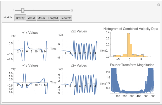
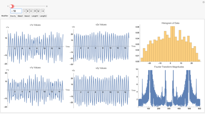
Now that we can plot the double pendulum simulation variables over time, we can use Manipulate to interactively explore how different input parameters affect the system. Varying parameters such as initial angles and velocities reveals the system’s sensitivity to changes. Additionally, tests like the Fourier Magnitudes test help analyze the frequency components of the system’s motion, indicating whether the behavior is periodic or chaotic. Histograms of variables like angular displacement and velocity show the distribution of values, helping to assess whether the system exhibits predictable patterns or random behavior. Together, these tools provide a deeper understanding of the system’s dynamics.
In[]:=
Clear[g,x1,y1,x2,y2,λ1,λ2];modifierRange={1,10};modifierMapping=<|"Gravity"->g,"Mass1"->Subscript[m,1],"Mass2"->Subscript[m,2],"Length1"->Subscript[l,1],"Length2"->Subscript[l,2]|>;parameterManipulate=Manipulate[Module[{params,ics,aeqns,soldp,v1x,v1y,v2x,v2y,tValues,v1xValues,v1yValues,v2xValues,v2yValues,combinedData,fourierTransform},(*Definetimevalues*)tValues=Range[0,15,0.1];(*Initializeparameters*)params=<|g->9.81,Subscript[m,1]->1,Subscript[m,2]->1,Subscript[l,1]->1,Subscript[l,2]->1|>;(*Updatetheselectedparameter*)modifier=modifierMapping[Modifier];params[modifier]=i;params=Normal[params];(*Definealgebraicanddifferentialequations*)aeqns={x1[t]^2+y1[t]^2==Subscript[l,1]^2,(x2[t]-x1[t])^2+(y2[t]-y1[t])^2==Subscript[l,2]^2};deqns={x1''[t]==-λ1[t]x1[t]-gSubscript[m,1],y1''[t]==-λ1[t]y1[t],x2''[t]==-λ2[t](x2[t]-x1[t]),y2''[t]==-λ2[t](y2[t]-y1[t])-gSubscript[m,2]};(*Defineinitialconditions*)ics={x1[0]==1+0.1i,y1[0]==0,x1'[0]==0,y1'[0]==0,x2[0]==1,y2[0]==-1,x2'[0]==0,y2'[0]==0};(*Solvethesystemofequations*)soldp=Quiet[First[NDSolve[{deqns,aeqns,ics}/.params,{x1,y1,x2,y2,λ1,λ2},{t,0,15},Method->{"IndexReduction"->{"Pantelides","ConstraintMethod"->"Projection"}}]]];(*Computevelocities*)v1x[t_]:=Evaluate[D[x1[t],t]/.soldp];v1y[t_]:=Evaluate[D[y1[t],t]/.soldp];v2x[t_]:=Evaluate[D[x2[t],t]/.soldp];v2y[t_]:=Evaluate[D[y2[t],t]/.soldp];v1xValues=v1x/@tValues;v1yValues=v1y/@tValues;v2xValues=v2x/@tValues;v2yValues=v2y/@tValues;(*CombinedataandcomputeFourierTransform*)combinedData=Flatten[{v1xValues,v1yValues,v2xValues,v2yValues}];fourierTransform=Fourier[combinedData];(*Generateplots*)Row[{Column[{ListLinePlot[Transpose[{tValues,v1xValues}],PlotLabel->"v1x Values",AxesLabel->{"Time","v1x"},ImageSize->Medium],ListLinePlot[Transpose[{tValues,v1yValues}],PlotLabel->"v1y Values",AxesLabel->{"Time","v1y"},ImageSize->Medium]}],Column[{ListLinePlot[Transpose[{tValues,v2xValues}],PlotLabel->"v2x Values",AxesLabel->{"Time","v2x"},ImageSize->Medium],ListLinePlot[Transpose[{tValues,v2yValues}],PlotLabel->"v2y Values",AxesLabel->{"Time","v2y"},ImageSize->Medium]}],Column[{Histogram[combinedData,20,"Probability",PlotLabel->"Histogram of Combined Velocity Data",ImageSize->Medium],ListLinePlot[Abs[fourierTransform],PlotLabel->"Fourier Transform Magnitudes",ImageSize->Medium]}]}]],{i,modifierRange[[1]],modifierRange[[2]],1},{Modifier,Keys[modifierMapping]},SaveDefinitions->True];manipulateToGif[parameterManipulate,"parameter_manipulate"]
Out[]=
Results of Optimization Testing
Results of Optimization Testing
We found that changing the mass provides the most change in output randomness, followed closely by gravity and then by pendulum rod length. Interestingly, a negative integer gravity (while not physically possible), leads to slightly better results in output when compared to its corresponding positive integer. Finally, we found a gravity of -10 significantly increases output randomness, visible on the histogram and on the fourier magnitudes test, but we have yet to figure out the exact reason.
In[]:=
Creating the ChaoticHash Function
Creating the ChaoticHash Function
By harnessing the abilities of this double pendulum simulation, we can now develop this hash function fully.
Selecting Simulation Parameters
Selecting Simulation Parameters
The first step in the ChaoticHash function involves deriving the physical parameters of the double pendulum—masses and lengths of its rods—from the input string. This process begins by converting the input string into its corresponding ASCII values. ASCII (American Standard Code for Information Interchange) is a character encoding standard that assigns numerical values to letters, digits, and symbols, allowing computers to process text efficiently. Each character is represented by a unique number (e.g., ‘A’ = 65, ‘a’ = 97), which is widely used in computing and cryptography. These ASCII values are then processed to determine specific positions within the array using an increment that is relatively prime to the length of the string. This ensures that the selection process cycles through all possible positions without repetition, making the parameter selection deterministic and sensitive to the input string.
The selected ASCII values are normalized to a range between 0 and 1, ensuring they can be mapped consistently to the desired physical ranges. The normalized values are then scaled to define the pendulum’s masses and lengths within predetermined ranges of 0.5 to 5.0 kilograms and meters, respectively. This mapping process ensures that even small changes in the input string result in unique and corresponding changes in the physical parameters of the simulation.
In[]:=
SelectSimulationParameters[input_]:=Module[{},asciiValues=ToCharacterCode[input];length=Length[asciiValues];increment=First[Select[Range[2,Max[2,length-1]],CoprimeQ[#,length]&]];positions=Mod[Range[0,length-1]*increment,length]+1;selectedValues=asciiValues[[positions]];normalizedValues=Rescale[selectedValues,{0,255},{0,1}];mMin=0.5;mMax=5.0;lMin=0.5;lMax=5.0;m1=mMin+Mean[Take[normalizedValues,{1,-1,4}]]*(mMax-mMin);m2=mMin+Mean[Take[normalizedValues,{2,-1,4}]]*(mMax-mMin);l1=lMin+Mean[Take[normalizedValues,{3,-1,4}]]*(lMax-lMin);l2=lMin+Mean[Take[normalizedValues,{4,-1,4}]]*(lMax-lMin);{m1,m2,l1,l2}];
For example, this helper function turns a given string into some parameters to be used in the double pendulum simulation below.
In[]:=
SelectSimulationParameters["ewfrg"]
Out[]=
{2.39706,2.3,2.31765,2.6}
Creating Initial Conditions
Creating Initial Conditions
Once the pendulum’s physical parameters are established, its initial conditions are defined. The pendulum is initialized with fixed starting angles of 90 degrees, representing a vertical downward position. Angular velocities are set to zero, ensuring the pendulum starts from rest. Using trigonometric functions, the positional coordinates of the pendulum arms are calculated based on their lengths and initial angles. These coordinates define the starting positions of both pendulums in the simulation. Additionally, the corresponding velocity components for each arm are computed, ensuring a complete description of the pendulum’s initial state. These initial conditions provide the starting point for simulating the chaotic motion.
In[]:=
CreateInitialConditions[]:=Module[{},theta1=Pi/2;theta2=Pi/2;omega1=0;omega2=0;x1Init=l1*Sin[theta1];y1Init=-l1*Cos[theta1];x1DotInit=l1*omega1*Cos[theta1];y1DotInit=l1*omega1*Sin[theta1];x2Init=x1Init+l2*Sin[theta2];y2Init=y1Init-l2*Cos[theta2];x2DotInit=x1DotInit+l2*omega2*Cos[theta2];y2DotInit=y1DotInit+l2*omega2*Sin[theta2];{x1Init,y1Init,x1DotInit,y1DotInit,x2Init,y2Init,x2DotInit,y2DotInit}];
Calling the function here creates the initial condition for the DP simulation.
In[]:=
CreateInitialConditions[]
Out[]=
{2.23529,0.,0.,0.,4.21765,0.,0.,0.}
Solving the Double Pendulum Simulation
Solving the Double Pendulum Simulation
This part of the function uses largely the same code as before to solve the double pendulum simulation using the two mass values, two lengths values, and the initial conditions.
In[]:=
SolveConstraintDPSimulation[{m1_,m2_,l1_,l2_},initialConditions_]:=Module[{},g=-10;params={Subscript[m,1]m1,Subscript[m,2]m2,Subscript[l,1]l1,Subscript[l,2]l2,gg};deqns={Subscript[m,1]x1''[t]==(λ1[t]/Subscript[l,1])x1[t]-(λ2[t]/Subscript[l,2])(x2[t]-x1[t]),Subscript[m,1]y1''[t]==(λ1[t]/Subscript[l,1])y1[t]-(λ2[t]/Subscript[l,2])(y2[t]-y1[t])-Subscript[m,1]g,Subscript[m,2]x2''[t]==(λ2[t]/Subscript[l,2])(x2[t]-x1[t]),Subscript[m,2]y2''[t]==(λ2[t]/Subscript[l,2])(y2[t]-y1[t])-Subscript[m,2]g};aeqns={x1[t]^2+y1[t]^2==Subscript[l,1]^2,(x2[t]-x1[t])^2+(y2[t]-y1[t])^2==Subscript[l,2]^2};soldp=First[NDSolve[{deqns,aeqns,initialConditions}/.params,{x1,y1,x2,y2,λ1,λ2},{t,0,15},Method{"IndexReduction"{"Pantelides","ConstraintMethod""Projection"}}]];soldp];
The function SolveConstraintDPSimulation outputs a solution to the system of differential equations governing the motion of a double pendulum under constraints. Specifically, it returns an interpolating function that represents the time evolution of the pendulum’s positions (x1, y1, x2, y2) and the constraint forces (λ1, λ2) over a specified time interval.
As a side note, even though a negative integer value for g is not possible, we found that this value of g makes the outputs of the function as random as possible through our randomness optimization tests mentioned earlier.
Extracting the Simulation Data
Extracting the Simulation Data
This part extracts the position values and velocity values (by taking the derivative with respect to time) throughout the double pendulum’s motion to be used in the hashing process.
In[]:=
ExtractSimulationData[soldp_]:=Module[{},(*ExtractData*)tValues=Range[0,15,0.05];x1Values=x1/.soldp/.t#&/@tValues;y1Values=y1/.soldp/.t#&/@tValues;x2Values=x2/.soldp/.t#&/@tValues;y2Values=y2/.soldp/.t#&/@tValues;v1xValues=(D[x1[t],t]/.soldp)/.t#&/@tValues;v1yValues=(D[y1[t],t]/.soldp)/.t#&/@tValues;v2xValues=(D[x2[t],t]/.soldp)/.t#&/@tValues;v2yValues=(D[y2[t],t]/.soldp)/.t#&/@tValues;Flatten[{x1Values,y1Values,x2Values,y2Values,v1xValues,v1yValues,v2xValues,v2yValues}]];
Generating the Hash
Generating the Hash
The chaotic motion data generated from the simulation is then processed to create the final hash. The simulation outputs are flattened and combined into a single dataset representing the positional and velocity changes of the pendulum over time. This data is normalized to ensure it falls within a consistent range, making it suitable for further processing. The normalized data is converted into integers and organized into a byte array. Finally, this processed data is hashed using the SHA256 algorithm to produce the output hash.
In[]:=
ChaoticHash[inputString_String]:=Module[{asciiValues,length,increment,positions,selectedValues,m1,m2,l1,l2,theta1,theta2,omega1,omega2,initialConditions,params,tValues,soldp,v1xValues,v1yValues,v2xValues,v2yValues,x1Values,y1Values,x2Values,y2Values,combinedData,hashOutput,g,mMin,mMax,lMin,lMax},{m1,m2,l1,l2}=SelectSimulationParameters[inputString];{x1Init,y1Init,x1DotInit,y1DotInit,x2Init,y2Init,x2DotInit,y2DotInit}=CreateInitialConditions[];initialConditions={x1[0]==x1Init,y1[0]==y1Init,x1'[0]==x1DotInit,y1'[0]==y1DotInit,x2[0]==x2Init,y2[0]==y2Init,x2'[0]==x2DotInit,y2'[0]==y2DotInit};soldp=SolveConstraintDPSimulation[{m1,m2,l1,l2},initialConditions];combinedData=ExtractSimulationData[soldp];normalizedData=Rescale[combinedData,MinMax[combinedData],{0,255}];integerData=Round[normalizedData];byteData=IntegerDigits[integerData,256,1];byteArray=FromDigits[Flatten[byteData],256];hashOutput=IntegerString[Hash[byteArray,"SHA256"],16,64];hashOutput]
By hashing this data using SHA256, the function combines the unpredictability of chaos with the strength of a standard cryptographic algorithm. As we will see later, all the preprocessing with the double pendulum simulation will make this chaotic hash function outperform SHA256 on a variety of cryptographic tests.
The ChaoticHash function produces a hexadecimal string as its output, similar to many widely-used cryptographic hash functions like SHA256. This hexadecimal string represents the processed result of the chaotic double pendulum simulation, normalized and further hashed using SHA256.
In[]:=
ChaoticHash["Hello World!"]
Out[]=
ba984548ac3042ca6a0a9cf90670e2480974741690909ff80177de1269ec291d
This output is a fixed-length string of 64 hexadecimal characters, corresponding to 256 bits of data. The fixed size ensures that the hash function’s output is consistent regardless of the input length, a critical property for applications like cryptographic hashing, data verification, and key generation. The high sensitivity of the ChaoticHash function ensures that even the smallest change in the input string would produce a drastically different hexadecimal output, maintaining the unpredictability and uniqueness required for hashing.
Here, we change the capital letter “H” of the beginning of “Hello World!” to a lowercase “h” but it still produces a vastly difference output compared to the output for the first string.
In[]:=
ChaoticHash["hello World!"]
Out[]=
eef8a4bc9619aba737f582e3378c00819fc1bb13a30126b6465eff442049c285
Comparisons to Other Hash Functions
Comparisons to Other Hash Functions
To evaluate the ChaoticHash function, it is important to compare it to widely-used standard hash functions such as MD5, SHA1, SHA224, and SHA256. These comparisons provide a clear understanding of how ChaoticHash performs in terms of key properties like sensitivity to input changes, uniformity in bit distributions, and adherence to statistical measures of randomness. Standard hash functions are commonly used in applications like cryptography, data verification, and distributed systems, making them useful benchmarks for assessing new hashing methods. By examining metrics such as Hamming distances, bit distributions, and results from the Pearson chi-square test, we can better understand how ChaoticHash measures up and whether it can serve as a viable alternative in practical applications.
Hamming Distances
Hamming Distances
Hash functions are designed to produce outputs that are highly sensitive to even the smallest changes in input. This sensitivity ensures that two inputs differing by just a single character generate drastically different hash values, an essential property for cryptographic and other practical applications. A useful way to quantify this sensitivity is through the Hamming distance, which measures the number of differing bits between two binary outputs.
To compute the Hamming distance, we implemented a function, HammingDistanceHex, that converts two hexadecimal hash outputs into their binary equivalents and calculates the total number of bits that differ.
HammingDistanceHex[hash1_,hash2_]:=Module[{bin1,bin2},bin1=IntegerDigits[FromDigits[hash1,16],2,256];bin2=IntegerDigits[FromDigits[hash2,16],2,256];Total[Abs[bin1-bin2]]]
Here is an example of the Hamming Distance function finding the distance between any two strings:
In[]:=
HammingDistanceHex["q","qqq"]
Out[]=
6
Using this function, we generated two similar input strings: “TestString” and “testString”. These strings differ by only a single character, making them ideal for testing the sensitivity of hash functions. The hash outputs for these inputs were computed using seven different functions: MD5, SHA1, SHA224, SHA256, Adler32, CRC32, and the custom chaotic hash function (referred to as “ChaoticHash”). By comparing the hamming distance between these seven functions, we can see how our hash function based on double pendulum motion measures up to more widely used hash functions.
We lay out our strings and hash functions:
In[]:=
testStrings={"TestString","testString"};customHashes=ChaoticHash/@testStrings;hashFunctions={"MD5","SHA1","SHA224","SHA256","Adler32","CRC32"};
We compute the Hamming Distances and display the results:
In[]:=
hammingDistances=Map[Function[func,hashes=IntegerString[Hash[#,func],16]&/@testStrings;dist=HammingDistanceHex[hashes[[1]],hashes[[2]]];{func,dist}],hashFunctions];customDist=HammingDistanceHex[customHashes[[1]],customHashes[[2]]];hammingDistances=Append[hammingDistances,{"ChaoticHash",customDist}];Grid[Prepend[hammingDistances,{"Hash Function","Hamming Distance"}],Frame->All]
Out[]=
Hash Function | Hamming Distance |
MD5 | 65 |
SHA1 | 79 |
SHA224 | 112 |
SHA256 | 113 |
Adler32 | 3 |
CRC32 | 15 |
ChaoticHash | 118 |
Adler32 and CRC32, which are checksum algorithms rather than cryptographic hashes, unsurprisingly show very low Hamming distances of 3 and 15, respectively. MD5, despite being widely used historically, demonstrates pretty weak sensitivity, with a Hamming distance of only 65. SHA1 shows a little improvement, with a distance of 79. However, both SHA224 and SHA256, which are more modern cryptographic hash functions, exhibit stronger sensitivity, with distances of 112 and 113, respectively.
But our “ChaoticHash” function has by far the best sensitivity, with a Hamming distance of 118. This result demonstrates exceptional sensitivity to input changes, surpassing even SHA256. The double pendulum dynamics underlying its design appear to introduce significant randomness, ensuring that minor modifications in input produce outputs with substantial differences at the bit level.
Bit Distributions
Bit Distributions
Another important property of hash functions is how they utilize their output space. A good hash function should produce outputs that are not only sensitive to input changes but also exhibit uniformity in their bit distributions. This means the number of bits set to 1 and 0 should be balanced, ensuring the hash function leverages its full output space effectively.
To explore this property, we analyzed the bit distributions of hash outputs for several built-in hash functions—MD5, SHA1, SHA224, and SHA256—as well as the custom chaotic hash function (“ChaoticHash”). The analysis involved generating hash outputs for 500 randomly generated strings and calculating the total number of bits set to 1 in the binary representation of each hash output. Each string is randomly selected between 10 characters and 20 characters long and randomly sampled from uppercase letters, lowercase letters, and digits.
In[]:=
randomStrings500=Table[StringJoin[RandomChoice[CharacterRange["A","Z"]~Join~CharacterRange["a","z"]~Join~CharacterRange["0","9"],RandomInteger[{10,20}]]],{500}];
Once the test strings were prepared, the hash outputs were computed for four widely-used cryptographic hash functions: MD5, SHA1, SHA224, and SHA256. For each function, the hexadecimal outputs were converted into binary, and the total number of bits set to 1 was calculated.
computeBitCounts[hashFunc_]:=Module[{hashes,bitCounts},hashes=IntegerString[Hash[#,hashFunc],16]&/@randomStrings500;bitCounts=Total[IntegerDigits[FromDigits[#,16],2]]&/@hashes;bitCounts];hashFunctions={"MD5","SHA1","SHA224","SHA256"};bitCountsList500=Table[computeBitCounts[hashFunc,randomStrings500],{hashFunc,hashFunctions}];
In addition to the standard hash functions, I also analyzed the custom chaotic hash function (“ChaoticHash”). Since this function produces outputs differently, it was processed separately and then combined with the rest of the functions. (Note: the following code cells take a long time time to run due to the computational workload of double pendulum simulations.)
In[]:=
chaoticHashes500=ChaoticHash/@randomStrings500;chaoticBitCounts500=Total[IntegerDigits[FromDigits[#,16],2]]&/@chaoticHashes500;allBitCounts500=Append[bitCountsList500,chaoticBitCounts500];allHashFunctions500=Join[hashFunctions,{"ChaoticHash"}];
Finally, we created histograms to visualize the bit distribution for each hash function. Each histogram represents the frequency of outputs with different numbers of bits set to 1, providing a clear comparison of the bit usage across hash functions.
PanelHistogram500=Table[Histogram[allBitCounts500[[i]],PlotLabel->allHashFunctions500[[i]],AxesLabel->{"Bits Set to 1","Frequency"}],{i,Length[allBitCounts500]}];GraphicsGrid[Partition[PanelHistogram500,UpTo[2]],Spacings->{0.5,0.5}]
Out[]=
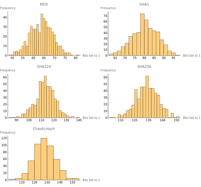
The resulting grid of histograms provides a visual representation of how each hash function distributes bits set to 1 in its outputs. MD5 and SHA1 exhibit narrower distributions compared to the other hash functions, with MD5 centered around 60–70 and SHA1 around 75–85. These distributions reflect their smaller output sizes and less effective utilization of bit space. In contrast, SHA224 and SHA256 display broader distributions, with SHA224 centered around 110–120 and SHA256 around 120–130, reflecting better randomness and more effective use of their larger bit spaces.
The custom chaotic hash function exhibits a behavior similar to that of SHA256 but with a slight shift toward higher values, centered around 125–135. This indicates a potential enhancement in randomness and uniformity due to the chaotic dynamics underlying its design. Its distribution not only matches but slightly exceeds SHA256 in bit utilization, suggesting it may achieve even stronger uniformity and unpredictability, essential traits for a practical hash function.
Assessing Uniformity with the Pearson Chi-Square Test
Assessing Uniformity with the Pearson Chi-Square Test
While histograms provide a visual understanding of the bit distributions in hash function outputs, a quantitative test can offer deeper insights into how well the distributions align with the expected uniformity. To achieve this, we conducted a Pearson chi-square test for each hash function, measuring how closely the observed bit distributions match a theoretical uniform distribution.
The Pearson chi-square test calculates a statistical p-value, which indicates whether the deviations from uniformity are significant. A low p-value suggests that the observed distribution deviates significantly from uniformity, while a high p-value indicates better alignment with a uniform distribution. For this test, the bit distributions computed earlier were used to perform the statistical analysis.
In[]:=
uniformityTestResults500=Table[{allHashFunctions500[[i]],PearsonChiSquareTest[allBitCounts500[[i]]]},{i,Length[allBitCounts500]}];Grid[Prepend[uniformityTestResults500,{"Hash Function","p-Value"}],Frame->All]
Out[]=
Hash Function | p-Value |
MD5 | 7.68344× -35 10 |
SHA1 | 2.18824× -21 10 |
SHA224 | 2.03294× -14 10 |
SHA256 | 3.13642× -9 10 |
ChaoticHash | 0.0038657 |
The results reveal that all of the standard hash functions tested—MD5, SHA1, SHA224, and SHA256—produced extremely low p-values, indicating significant deviations from uniformity. Among these, MD5 and SHA1 perform the worst, with p-values on the order of and , respectively. This outcome aligns with their older and less robust designs. SHA224 and SHA256 demonstrate some improvement, with higher (though still small) p-values, suggesting better but not perfect uniformity in their bit distributions.
-35
10
-21
10
In contrast, the chaotic hash function achieves a p-value of approximately 0.00387, which, while slightly below the conventional significance threshold of 0.05, represents a dramatic improvement over the standard hash functions. This result suggests that the chaotic dynamics underlying its design contribute significantly to achieving a more uniform bit distribution, reducing patterns or biases present in its output.
Conclusion & Future Work
Conclusion & Future Work
The ChaoticHash function introduces a new way of creating hash values by using the chaotic motion of a double pendulum. This approach is different from traditional hash functions like MD5 or SHA256, as it uses the unpredictability of chaotic systems to generate randomness. By simulating the behavior of the double pendulum and optimizing its parameters, the ChaoticHash function was designed to respond strongly to changes in input and produce outputs that are well-distributed and hard to predict through running some randomness optimization tests.
When comparing ChaoticHash to other hash functions, it showed some clear strengths. The Hamming distance tests revealed that ChaoticHash responds more strongly to small input changes than other functions, which is an important feature of a good hash function. The bit distribution analysis showed that ChaoticHash makes good use of its output space, producing balanced and unpredictable results. Finally, the Pearson chi-square test demonstrated that its outputs are closer to random and uniform than many of the other hash functions tested. However, a limitation of ChaoticHash is its computational efficiency, since its run-time is relatively higher than that of SHA-256 or other industry-standard hash functions.
Future work could focus on examining the scalability of ChaoticHash when applied to larger datasets and assessing its computational efficiency relative to traditional hash functions. Additional research could also investigate the use of other chaotic systems, such as Lorenz attractors or chaotic maps, to further refine the process of generating randomness. Improvements to the parameter optimization process in the double pendulum simulation could enhance the consistency and quality of the outputs. These directions would help further evaluate and improve the practical utility of ChaoticHash in a variety of applications.
Acknowledgement
Acknowledgement
We would like to thank Felipe Amorim, our mentor, for all his help and reassurance throughout the course of this project. Also, thanks to Eryn Gilliam for her help in checking our progress while we were working. And much appreciation to the Wolfram Emerging Leaders Program for this opportunity to explore this unique combination of our interests.
Helper Function for Animations
Helper Function for Animations
In[]:=
manipulateToGif[manipulate_,filename_String]:=AnimatedImage[Import[Export[filename<>".gif",manipulate]],ImageSize->Full];
References
References
CITE THIS NOTEBOOK
CITE THIS NOTEBOOK
Post-quantum hashing using chaotic double pendulum dynamics
by Wolfram Education Programs
Wolfram Community, STAFF PICKS, February 5, 2025
https://community.wolfram.com/groups/-/m/t/3381079
by Wolfram Education Programs
Wolfram Community, STAFF PICKS, February 5, 2025
https://community.wolfram.com/groups/-/m/t/3381079