Sometimes it is useful to have a function that smooths as well as interpolates data. In cases where the domain of the data is well defined and it is not necessary to preserve the actual data points a Chebyshev polynomial approximation can be useful and quite accurate.
The algorithm below was adapted from Numerical Recipes and overloaded to take a variety of input patterns including functions. The output is a polynomial as a Function.
Data
volumeData1=;
The data for the examples below is minute volume data for the ten lowest volatility trading days for the SPY ETF between 31 March and 3 September 2021. The idea is to get a polynomial fit that smooths the data for each day to get an idea of the underlying function shape.
In[]:=
GraphicsGridPartitionDateListPlot#,&/@volumeData1,5,ImageSize->1000
Out[]=
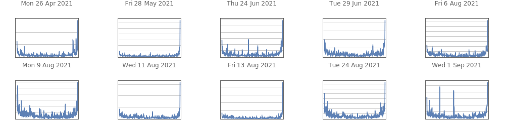
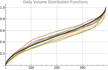
The data was changed from a volume per minute to accumulated volume divided by total volume to standardize the volume function to a distribution function of relative volume per trading minute of the day. The raw data gives the data for the end of the minute and there are 390 minutes per day. A zero volume at minute 0 was added to give a zero volume point before trading starts. Note that if you change the Method to “Hermite” you should apply N to the data, as it is in integers and the ChebyPoly algorithms are set up to support arbitrary precision. Note also that numerically integrating the data with Accumulate[] causes some smoothing.
The thick black line is that of an ArcSinDistribution which was suggested by the shape of the polynomial function.
Chebyshev Algorithms: Function Definitions
Chebyshev Algorithms: Function Definitions
Examples
Examples
In[]:=
volFns=ChebyPoly[Interpolation[Transpose[{Range[0,390],Accumulate[Join[{0},#[[All,2]]]/Total[#[[All,2]]]]}],Method->"Spline"],16]&/@volumeData1;gdfn=PlotEvaluate[#[t]&/@volFns],{t,0,390},;asin=PlotCDF[ArcSinDistribution[{0,390}],t],{t,0,390},;Show[gdfn,asin]
Out[]=
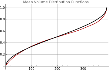
Here is the ArcSinDistribution compared to the average of the ten polynomial functions. The minute volume distribution accumulates more slowly, than the ArCSinDistribution but catches up rapidly in the final minutes of trading.
In[]:=
gdfn=PlotEvaluate[Mean[#[t]&/@volFns]],{t,0,390},;Show[gdfn,asin]
Out[]=
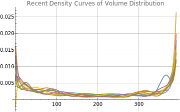
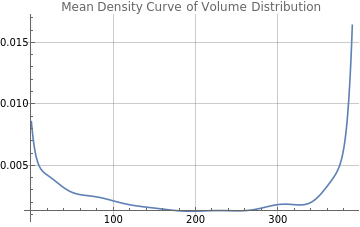
What I found interesting was that the fit to the relative volume by minute could be nicely modeled by the first derivative of the polynomial approximations.
In[]:=
PlotEvaluate[#'[t]&/@volFns],{t,0,390},
Out[]=
In[]:=
PlotEvaluate[Mean[#'[t]&/@volFns]],{t,0,390},
Out[]=
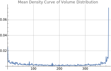
Here is what it looks like using Interpolation[].
In[]:=
volFns1=Interpolation[Transpose[{Range[0,390],Accumulate[Join[{0},#[[All,2]]]/Total[#[[All,2]]]]}],Method->"Spline"]&/@volumeData1;PlotEvaluate[Mean[#'[t]&/@volFns1]],{t,0,390},
Out[]=
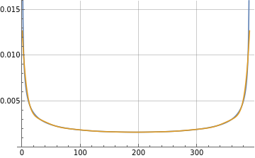
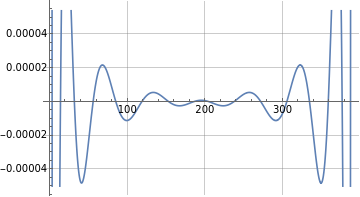
This compares the Chebyshev polynomial fit to the actual distribution function, using the same n = 16, then compares the first derivatives. Note that actual ArcSinDistribution density at points 0 and 390 would be infinite.
In[]:=
arcsinpoly=ChebyPoly[CDF[ArcSinDistribution[{0,390}],#]&,{0,390},16]//N;Plot{PDF[ArcSinDistribution[{0,390}],x],arcsinpoly'[x]},{x,0,390},Plot{PDF[ArcSinDistribution[{0,390}],x]-arcsinpoly'[x]},{x,0,390},
Out[]=
Out[]=
The volume data does not need to be scaled the polynomial approximation will still work.
In[]:=
Plot[ChebyPoly[Transpose[{Range[0,390],Join[{0},Accumulate[volumeData1[[-1]][[All,2]]]]}],{0,390},16][t],{t,0,390}]Plot[volFns[[-1]][t],{t,0,390}]
Out[]=
Out[]=
Lower degree polynomial fitting will smooth the data more but also eliminate higher slopes and frequencies in the data.
In[]:=
Plot[{ChebyPoly[Transpose[{Range[0,390],Join[{0},Accumulate[volumeData1[[-1]][[All,2]]]]}],{0,390},5][t],Interpolation[Transpose[{Range[0,390],Join[{0},Accumulate[volumeData1[[-1]][[All,2]]]]}]][t]},{t,0,390}]
Out[]=
Higher degree polynomials can run into precision problems, because of the large number of multiplications of the Chebyshev coefficients involved in converting the Chebyshev coefficients to polynomial coefficients. The routine ChebyEval reduces the number of multiplications greatly reducing the loss of precision. The second plot takes a while because of the oscillations caused by loss of precision.
In[]:=
Plot[ChebyPoly[Transpose[{Range[0,390],Join[{0},Accumulate[volumeData1[[-1]][[All,2]]]]}],{0,390},20][t],{t,0,390}]Plot[ChebyPoly[Transpose[{Range[0,390],Join[{0},Accumulate[volumeData1[[-1]][[All,2]]]]}],{0,390},24][t],{t,0,390}]
Out[]=
Out[]=
This computes each point using the Chebyshev coefficients and makes the plots directly from them rather than from the polynomials.
In[]:=
cc=ChebyCoeff[Interpolation[Transpose[{Range[0,390],Join[{0},Accumulate[volumeData1[[-1]][[All,2]]]]}],Method->"Spline"],{0,390},24]
Out[]=
{3.53249×,1.48248×,-576176.,1.8615×,256122.,391981.,92552.,120605.,224957.,279792.,121613.,-107275.,94357.9,42515.7,-79013.,98781.5,60757.7,41063.2,-69714.6,261.566,29323.8,12466.7,-40228.3,62881.1}
7
10
7
10
6
10
In[]:=
Plot[ChebyEval[cc,{0,390},t],{t,0,390}]
Out[]=
The first derivative may also be calculated more efficiently directly from the Chebyshev coefficients than from the first derivative of the polynomial.
In[]:=
cp24=ChebyPoly[Transpose[{Range[0,390],Join[{0},Accumulate[volumeData1[[-1]][[All,2]]]]}],{0,390},24]cder=ChebyDer[cc,{0,390}];Plot[{cp24'[t],ChebyEval[cder,{0,390},t]},{t,0,390}]
Out[]=
147592.+626127.#1-163825.+24977.6-2128.19+115.381-4.28695+0.11453-0.00227669+0.0000345423-4.07703×+3.79673×-2.8177×+1.67724×-8.0325×+3.09415×-9.54876×+2.34119×-4.49651×+6.61487×-7.19226×+5.4433×-2.55944×+5.62839×&
2
#1
3
#1
4
#1
5
#1
6
#1
7
#1
8
#1
9
#1
-7
10
10
#1
-9
10
11
#1
-11
10
12
#1
-13
10
13
#1
-16
10
14
#1
-18
10
15
#1
-21
10
16
#1
-23
10
17
#1
-26
10
18
#1
-29
10
19
#1
-32
10
20
#1
-35
10
21
#1
-38
10
22
#1
-42
10
23
#1
Out[]=