This project explores methods to optimize railroad placement. The first half of my project decides the railroad connections required to connect a list of cities based on various parameters, such as distance, elevation change, and population. The second half of my project is a pathfinding function between two points on a GridGraph, where elevation change is the only parameter.
Introduction
Introduction
Effective train lines increase accessibility, economic opportunities, and provide an efficient method of transport.
My project intends to find the optimal path to connect multiple locations using graphs and Dijkstra’s algorithm. Dijkstra’s algorithm is a pathfinding algorithm which finds the shortest path between two vertices. The graphs visualize connections between multiple locations, where locations are represented by vertices and edges represent the connections between vertices. Edges can have weight values, such as distance or other parameters. Higher edge weight values are considered more “costly” or less desirable to travel than lower edge weight values. Algorithms such as FindSpanningTree find the minimum connections required to connect all vertices, while trying to reduce edge weight.
(Vertices are also commonly referred to as nodes, though I will only use the term vertices).
I also encourage any reader to download this notebook for more readable code and so the graphs can be properly resized .
Deciding Railroad Connections
Deciding Railroad Connections
Basic Graph of City Connections
Basic Graph of City Connections
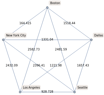
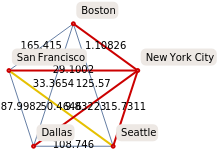
The basic version of the “railroad route” graph creates every possible connection between each city and includes edge weights.
cityPairs5 returns every possible pairing between the cities listed.
cityPairsConnections uses pattern matching to convert the city pairs into the format required for graphing.
cityPairDists returns the distance between each pair of cities.
cityPairsConnections uses pattern matching to convert the city pairs into the format required for graphing.
cityPairDists returns the distance between each pair of cities.
In[]:=
cityPairs5=Subsets,,,,,{2};cityPairsConnections=Cases[cityPairs5,{a_,b_}->ab];cityPairDists=QuantityMagnitude/@GeoDistance@@@cityPairs5;
While each edge of the graph is labeled with an edge weight based on the distance between the two vertices, or cities, the edge weights are not otherwise used in the basic graph.
In[]:=
basicGraph=Graph[cityPairsConnections,EdgeWeight->cityPairDists,EdgeLabels->"EdgeWeight",VertexLabels->Automatic]
Out[]=
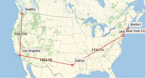
FindSpanningTree finds the least amount of edges which can be used to connect all the vertices, while taking any edge weights into account.
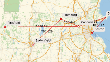
GeoGraphPlot is able to plot the graph on a map as my graph’s vertices are city entities, so no manual input of coordinates are required.
GeoGraphPlot is able to plot the graph on a map as my graph’s vertices are city entities, so no manual input of coordinates are required.
In[]:=
GeoGraphPlot[FindSpanningTree[basicGraph]]
Out[]=
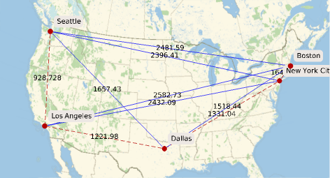
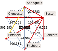
The following graphic shows the initial graph’s edges in blue and the edges selected by FindSpanningTree in red, dashed lines.
In[]:=
GeoGraphPlot[HighlightGraph[basicGraph,FindSpanningTree[basicGraph,EdgeWeight->cityPairDists]],EdgeStyle->Blue]
Out[]=
In[]:=
GraphDistancebasicGraph,,
Out[]=
2481.59
In[]:=
GraphDistanceFindSpanningTree[basicGraph],,
Out[]=
3646.16
Though FindSpanningTree greatly reduces the number of edges and thus “train tracks to be laid”, it can significantly increase the distance which must be traveled between two points. For example, travel distance from Seattle to Boston increases by 1164.57 miles, from 2481.59 miles for a direct connection to 3646.16 miles after FindSpanningTree. Thus, I created a function to help the user decide which railroad connection to build next, to “counteract” the increased distance from FindSpanningTree, which prioritizes minimizing edges over reducing travel distance in some cases.
Furthermore, edge weights other than distance are considered when constructing railroads, so I include city population and elevation change in the edge weights.
Furthermore, edge weights other than distance are considered when constructing railroads, so I include city population and elevation change in the edge weights.
cityConnectionGraphs input must be a list of city entities.
maxGeoElevPieces is the maximum amount of “pieces” a line can be split into. The pieces are points for which GeoElevationData is returned.
The amount of pieces any line between 2 cities will be split into is less than or equal to maxGeoElevpieces, where each piece has the same scale.
The longest distance is divided by maxGeoElevPieces, deciding the scale for the rest of function and reducing computing time.
Dividing the populations by 20,000 is to reduce the population numbers when being inputted into the edge weights
Function with Multiple EdgeWeight Parameters
Function with Multiple EdgeWeight Parameters
In[]:=
cityConnectionGraphs[x_,maxGeoElevPieces_:40]:=Module[{fxCityPairs=Subsets[x,{2}],fxCityPairDist,scaleFromMaxPieces,poplsOf2Locations,fxNEWCityPairMaxElevationDiff,fxNEWCityPairDistandElevDiffandPopl,fxGraphCityPairs,fxBasicGraph,fxOGOverSpanningTree,fxSpanningTree,fxSuggestNewRailroad},fxCityPairDist=QuantityMagnitude/@GeoDistance@@@fxCityPairs;scaleFromMaxPieces=Divide[Sort[fxCityPairDist][[Length[fxCityPairs]]],maxGeoElevPieces];poplsOf2Locations=Cases[fxCityPairs,{a_,b_}->Divide[QuantityMagnitude[EntityValue[a,"Population"]]+QuantityMagnitude[EntityValue[b,"Population"]],20000]];fxNEWCityPairMaxElevationDiff=Table[maxElevationDifference[i,scaleFromMaxPieces],{i,fxCityPairs}];fxNEWCityPairDistandElevDiffandPopl=Table[Divide[fxCityPairDist[[z]]+fxNEWCityPairMaxElevationDiff[[z]],poplsOf2Locations[[z]]],{z,1,Length[fxCityPairDist]}];fxGraphCityPairs=Cases[fxCityPairs,{a_,b_}->ab];fxBasicGraph=Graph[fxGraphCityPairs,EdgeWeight->fxNEWCityPairDistandElevDiffandPopl,EdgeLabels->"EdgeWeight",VertexLabels->"Name"];fxOGOverSpanningTree=Table[fxCityPairDist[[a]]/Table[GraphDistance[FindSpanningTree[fxBasicGraph],fxCityPairs[[All,1]][[a]],fxCityPairs[[All,2]][[a]],Method->"Dijkstra"],{a,1,Length[fxCityPairs]}][[a]],{a,1,Length[fxCityPairs]}];fxSpanningTree=GeoGraphPlot[FindSpanningTree[fxBasicGraph],ImageSize->Medium];fxSuggestNewRailroad=HighlightGraph[fxBasicGraph,{FindSpanningTree[fxBasicGraph],{Keys[Sort[AssociationThread[fxGraphCityPairs,fxOGOverSpanningTree]]][[1]]}},GraphHighlightStyle"Thick"];<|"Minimum Railroad Connection"->fxSpanningTree,"Suggested Railroad to Build Next (in yellow)"->fxSuggestNewRailroad,"Scale (miles) used to find Elevation Data"->scaleFromMaxPieces|>]
maxElevationDifference finds the elevation change between the highest and lowest elevation points on a line.
This is by taking the GeoElevationData of points spaced evenly on a line between two cities.
maxGeoElevPieces in the function above determines the scale, which is inputted into maxElevationDifference.
This is by taking the GeoElevationData of points spaced evenly on a line between two cities.
maxGeoElevPieces in the function above determines the scale, which is inputted into maxElevationDifference.
In[]:=
maxElevationDifference[x_List,scale_:10]:=Module[{piecesForCustomScale=Divide[QuantityMagnitude[GeoDistance[x]],scale],x1,y1,x2,y2,xValsLine,yValsLine,elevationList,elevationChange},{{x1,y1},{x2,y2}}=EntityValue[x,"Coordinates"];xValsLine=Table[x1+a,{a,0,x2-x1,(x2-x1)/piecesForCustomScale}];yValsLine=Table[y1+b,{b,0,y2-y1,(y2-y1)/piecesForCustomScale}];elevationList=QuantityMagnitude[GeoElevationData[GeoPosition[Transpose[{xValsLine,yValsLine}],1]]];elevationChange=Sort[elevationList][[Length[elevationList]]]-Sort[elevationList][[1]]]
Example Graphs With Different EdgeWeight Parameters
Example Graphs With Different EdgeWeight Parameters
In[]:=
cityConnectionGraphs,,,,,,20
Out[]=
Minimum Railroad Connection
,Suggested Railroad to Build Next (in yellow)
,Scale (miles) used to find Elevation Data6.20441
A flaw in my function is that some city connections are over water, which is not realistic for railroads.
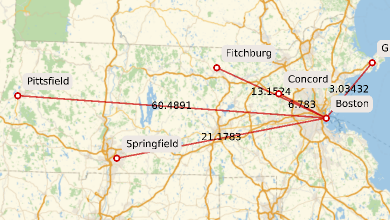
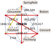
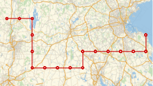
Including population as a parameter in the edge weights creates a more intuitive graph which loosely resembles the Massachusetts commuter rail.
For perspective, the “same” graph made without considering population would look like this:
Including population as a parameter in the edge weights creates a more intuitive graph which loosely resembles the Massachusetts commuter rail.
For perspective, the “same” graph made without considering population would look like this:
Identical to the function above, only with the population parameter removed.
In[]:=
cityConnectionGraphNoPopulation[x_,maxGeoElevPieces_:40]:=Module[{fxCityPairs=Subsets[x,{2}],fxCityPairDist,scaleFromMaxPieces,fxNEWCityPairMaxElevationDiff,fxNEWCityPairDistandElevDiff,fxGraphCityPairs,fxBasicGraph,fxOGOverSpanningTree,fxSpanningTree,fxSuggestNewRailroad},fxCityPairDist=QuantityMagnitude/@GeoDistance@@@fxCityPairs;scaleFromMaxPieces=Divide[Sort[fxCityPairDist][[Length[fxCityPairs]]],maxGeoElevPieces];fxNEWCityPairMaxElevationDiff=Table[maxElevationDifference[i,scaleFromMaxPieces],{i,fxCityPairs}];fxNEWCityPairDistandElevDiff=Table[fxCityPairDist[[z]]+fxNEWCityPairMaxElevationDiff[[z]],{z,1,Length[fxCityPairDist]}];fxGraphCityPairs=Cases[fxCityPairs,{a_,b_}->ab];fxBasicGraph=Graph[fxGraphCityPairs,EdgeWeight->fxNEWCityPairDistandElevDiff,EdgeLabels->"EdgeWeight",VertexLabels->"Name"];fxOGOverSpanningTree=Table[fxCityPairDist[[a]]/Table[GraphDistance[FindSpanningTree[fxBasicGraph],fxCityPairs[[All,1]][[a]],fxCityPairs[[All,2]][[a]],Method->"Dijkstra"],{a,1,Length[fxCityPairs]}][[a]],{a,1,Length[fxCityPairs]}];fxSpanningTree=GeoGraphPlot[FindSpanningTree[fxBasicGraph],ImageSize->Medium];fxSuggestNewRailroad=HighlightGraph[fxBasicGraph,{FindSpanningTree[fxBasicGraph],{Keys[Sort[AssociationThread[fxGraphCityPairs,fxOGOverSpanningTree]]][[1]]}},GraphHighlightStyle"Thick"];<|"Minimum Railroad Connection"->fxSpanningTree,"Suggested Railroad to Build Next (in yellow)"->fxSuggestNewRailroad,"Scale (miles) used to find Elevation Data"->scaleFromMaxPieces|>]
This graph has the same Massachusetts towns/cities as vertices, but only distance and elevation change are considered in the edge weights.
In[]:=
cityConnectionGraphNoPopulation,,,,,,20
Out[]=
Minimum Railroad Connection
,Suggested Railroad to Build Next (in yellow)
,Scale (miles) used to find Elevation Data6.20441
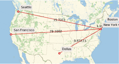
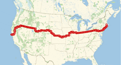
This graph is over a larger distance and considers all three parameters of distance, elevation change, and population.
In[]:=
cityConnectionGraphs,,,,
Out[]=
Minimum Railroad Connection
,Suggested Railroad to Build Next (in yellow)
,Scale (miles) used to find Elevation Data67.2116
In “Suggested Railroad to Build Next”, the yellow line is the next railroad suggested to be built, while lines highlighted red show the edges chosen by FindSpanningTree.
The new edge weight values are (distance in miles + elevation change in feet)/population divided by 20,000. The new edge weight function prioritizes population over parameters such as distance. This may not be the optimal ratio between all the parameters, though it can easily be customized.
The new edge weight values are (distance in miles + elevation change in feet)/population divided by 20,000. The new edge weight function prioritizes population over parameters such as distance. This may not be the optimal ratio between all the parameters, though it can easily be customized.
Pathfinding between Two Locations to Minimize Elevation Change
Pathfinding between Two Locations to Minimize Elevation Change
After determining which railroad connections to build, our new goal is to build a function which can find the shortest path between two points on a grid graph of elevation data.
Wolfram Language has the built in function GeoElevationData, which gives the elevation data in a grid format of latitudes and longitudes.
We approximate the geographic elevation between two cities as a GridGraph where each vertex has elevation data; part of its coordinate triple {latitude, longitude, elevation}.
Although this method reduces precision, it greatly improves the time it takes to run the functions.
Therefore, we control the GridGraph dimensions using the built in option GeoZoomLevel. GeoZoomLevel -> 1 is the lowest resolution and will have reduced dimensions, while GeoZoomLevel -> 12 is the highest resolution and would be computationally intensive to run.
The first item in the output list is the suggested zoom level to be inputted. The suggested zoom level is the highest resolution which still fulfils the requirements of having dimensions below 100 by 100.
Deciding Graph Dimensions
Deciding Graph Dimensions
In[]:=
helpMeDecideZoomLevel[twoLocations_List]:=Module[{fxminlat,fxmaxlat,fxminlon,fxmaxlon,dimensionList,zoomGrid,message,zoomWDimensions,dimensionCases,zoomLevel},{{fxminlat,fxmaxlat},{fxminlon,fxmaxlon}}=GeoBounds[twoLocations];dimensionList=Table[Dimensions[GeoElevationData[{{fxminlat,fxminlon},{fxmaxlat,fxmaxlon}},GeoZoomLevel->i]],{i,1,8}];zoomGrid=Grid[{Thread["ZoomLevel"->Range[8]],dimensionList},Frame->All,ItemStyle->FontSize->16];message=Style["Dimensions smaller than {100,100} help to reduce computing time. Please pick the Zoom Level accordingly.",Bold,Red];zoomWDimensions=Thread[Range[8]->dimensionList];dimensionCases=Cases[zoomWDimensions,HoldPattern[_->{a_/;a<=100,b_/;b<=100}]];zoomLevel=First@Keys[Association[Sort[dimensionCases][[Length[dimensionCases]]]]];{zoomLevel,zoomGrid,message}]
In[]:=
helpMeDecideZoomLevel,
Out[]=
6,
,Dimensions smaller than {100,100} help to reduce computing time. Please pick the Zoom Level accordingly.
ZoomLevel1 | ZoomLevel2 | ZoomLevel3 | ZoomLevel4 | ZoomLevel5 | ZoomLevel6 | ZoomLevel7 | ZoomLevel8 |
{2,4} | {3,6} | {5,12} | {9,24} | {16,46} | {32,91} | {63,180} | {124,359} |
Formatting GeoElevationData
Formatting GeoElevationData
geoCoordTriple is the input for the GridGraph of elevation data. geoCoordTriple finds the {latitude, longitude, elevation} of a bounding box created around 2 cities. GeoZoomLevel decides the graph dimensions and must be manually inputted as the second argument. You may follow the suggestions from the function helpMeDecideZoomLevel.
In[]:=
geoCoordTriple[twoLocations_List,zoomLevel_]:=Module[{fxminlat,fxmaxlat,fxminlon,fxmaxlon,elevData},{{fxminlat,fxmaxlat},{fxminlon,fxmaxlon}}=GeoBounds[twoLocations];elevData=GeoElevationData[{{fxminlat,fxminlon},{fxmaxlat,fxmaxlon}},Automatic,"GeoPosition",GeoZoomLevel->zoomLevel];elevData[[1]]]
In[]:=
geoCoordTriple,,2
Out[]=
{{{42.4008,-72.5977,116.154},{42.4008,-72.2461,205.211},{42.4008,-71.8945,215.068},{42.4008,-71.543,68.1292},{42.4008,-71.1914,14.4197},{42.4008,-70.8398,-37.2072}},{{42.0622,-72.5977,35.6239},{42.0622,-72.2461,195.403},{42.0622,-71.8945,151.2},{42.0622,-71.543,70.2776},{42.0622,-71.1914,4.59615},{42.0622,-70.8398,-0.965399}},{{41.7236,-72.5977,55.0021},{41.7236,-72.2461,102.483},{41.7236,-71.8945,81.2403},{41.7236,-71.543,29.371},{41.7236,-71.1914,-26.2376},{41.7236,-70.8398,-28.7077}}}
Pathfinding over GridGraph
Pathfinding over GridGraph
Our goal is to minimize elevation change, which is why elevation change between vertices adjacent by 1 unit on the GridGraph serve as the edge weights, thus excluding diagonals. This is another way our model is only an approximation, but elimination of diagonal edges again saves computation time.
I would like to thank Dugan Hammock for his significant contributions to section.
The geoElevationGridGraph function’s GridGraph output is 3 dimensional as elevations are assigned to vertex weights, which puts elevation on the z axis of the GridGraph.
We use a rule to thread the GridGraph vertices, which are only integers, to a transposed and flattened list of latitude and longitude coordinates. This matches up the latitude and longitude coordinates to their index in the list.
The latitude and longitude coordinates must be transposed to match how GridGraph formats vertices.
Transposing the elevation data insures adjacency between vertices is correct, though the GridGraph visualization is not oriented the exact way the vertices are represented geographically.
FindShortestPath finds the shortest path between two points using Dijkstra’s algorithm. As the only edge weight for the GridGraph is elevation change, FindShortestPath seeks to minimize elevation change.
After we find the shortest path between two points, we can extract the edges using EdgeList.
As the edges are only connections between vertices, we can replace vertices with latitude and longitude coordinates, following our rule from before.
This way, we can transfer a path from the GridGraph onto a geographical map.
The GridGraph with elevations and the pathfinding between two points are in the same function for efficiency, as the pathfinding uses the same variables as the GridGraph generation.
In[]:=
geoElevationGridGraphNoLabels[geoElv_,ptA_,ptB_]:=Module[{dimensions,elevMatrix,elevList,latlonsMatrix,latlonsList,latlonsGeoPositions,graph,edges,edgeWeightList,graphVertCoords,latlonsIndexRule,graphPath,graphOnMap},dimensions=Dimensions[geoElv][[1;;2]];elevMatrix=geoElv[[All,All,3]];elevList=Flatten[Transpose[elevMatrix]];latlonsMatrix=geoElv[[All,All,{1,2}]];latlonsList=Flatten[Transpose[latlonsMatrix],1];latlonsGeoPositions=Table[GeoPosition[x],{x,latlonsList}];graph=GridGraph[dimensions];graphVertCoords=graph//GraphEmbedding;graphVertCoords=Map[Flatten,Transpose[{graphVertCoords,10Rescale[elevList]}]];edges=graph//EdgeList;edgeWeightList=Map[Function[edge,Abs[elevList[[edge[[1]]]]-elevList[[edge[[2]]]]]],edges];graph=GridGraph[dimensions,EdgeWeight->edgeWeightList,EdgeLabels->None,VertexWeight->Thread[Rule[Range[Times@@dimensions],elevList]],VertexCoordinates->graphVertCoords];Thread[Rule[Range[Times@@dimensions],elevList]];latlonsIndexRule=Thread[Rule[Range[Times@@dimensions],latlonsGeoPositions]];graphPath=HighlightGraph[graph,PathGraph[FindShortestPath[graph,ptA,ptB]]];graphOnMap=GeoGraphPlot[Replace[PathGraph[FindShortestPath[graph,ptA,ptB]]//EdgeList,latlonsIndexRule,2]];{graph,graphPath,graphOnMap}]
Unfortunately, a limitation due to time constraints is that only points on the GridGraph can be inputted, and not actual coordinates.
In[]:=
geoElevationGridGraphNoLabelsgeoCoordTriple,,2,14,2060
Out[]=
 ,
, ,
,
This function is identical to the function above, apart from including the vertex labels from grid graph. The vertex labels can become messy for larger graphs with more vertices, which is I only suggest including labels for smaller graphs.
In[]:=
geoElevationGridGraphVertexLabels[geoElv_,ptA_,ptB_]:=Module[{dimensions,elevMatrix,elevList,latlonsMatrix,latlonsList,latlonsGeoPositions,graph,graphPath,edges,edgeWeightList,graphVertCoords,latlonsIndexRule,graphOnMap},dimensions=Dimensions[geoElv][[1;;2]];elevMatrix=geoElv[[All,All,3]];elevList=Flatten[Transpose[elevMatrix]];latlonsMatrix=geoElv[[All,All,{1,2}]];latlonsList=Flatten[Transpose[latlonsMatrix],1];latlonsGeoPositions=Table[GeoPosition[x],{x,latlonsList}];graph=GridGraph[dimensions];graphVertCoords=graph//GraphEmbedding;graphVertCoords=Map[Flatten,Transpose[{graphVertCoords,10Rescale[elevList]}]];edges=graph//EdgeList;edgeWeightList=Map[Function[edge,Abs[elevList[[edge[[1]]]]-elevList[[edge[[2]]]]]],edges];graph=GridGraph[dimensions,VertexLabels->Automatic,EdgeWeight->edgeWeightList,EdgeLabels->None,VertexWeight->Thread[Rule[Range[Times@@dimensions],elevList]],VertexCoordinates->graphVertCoords];Thread[Rule[Range[Times@@dimensions],elevList]];graphPath=HighlightGraph[graph,PathGraph[FindShortestPath[graph,ptA,ptB]]];latlonsIndexRule=Thread[Rule[Range[Times@@dimensions],latlonsGeoPositions]];graphOnMap=GeoGraphPlot[Replace[PathGraph[FindShortestPath[graph,ptA,ptB]]//EdgeList,latlonsIndexRule,2]];{graph,graphPath,graphOnMap}]
In[]:=
geoElevationGridGraphVertexLabelsgeoCoordTriple,,3,1,57
Out[]=
 ,
, ,
,
Limitations:
Limitations:
Unfortunately due to time constraints, my project has some limitations.
◼
For the Deciding Railroad Connections section of my project, the ratio between the different parameters included in the edge weights could be improved
◼
Currently, the GridGraph pathfinding does not distinguish between points on land and points on water. In the future, I would consider incorporating Open Street Map data to create a more realistic pathfinding function.
◼
In the current GridGraph, only 1 unit connections exist and there are no diagonal edges to reduce computing time. If there was more time available, I would have liked to incorporate the A* pathfinding algorithm and look for paths on a graph with much larger dimensions to improve accuracy. I would also like make a function to “round” the paths found by the geoElevationGridGraph function, as actual railroads are most efficient when horizontal curves are minimized.
◼
For the pathfinding part of the GridGraph function, only points on the GridGraph can be inputted, and not actual coordinates. In the future, I may use a rule to translate coordinates into points on the GridGraph for easier input.
Acknowledgements:
Acknowledgements:
A special thanks to my mentor Adam Millar, who guided me throughout my project, Dugan Hammock, who helped me greatly for the 2nd part of my project, and TAs Alisa, Zoya, and Logan for helping me with my code.
CITE THIS NOTEBOOK
CITE THIS NOTEBOOK
Optimizing train routes
by Claire Bian
Wolfram Community, STAFF PICKS, July 11, 2024
https://community.wolfram.com/groups/-/m/t/3217367
by Claire Bian
Wolfram Community, STAFF PICKS, July 11, 2024
https://community.wolfram.com/groups/-/m/t/3217367