Preface
Preface
In this paper, we explore the convergence properties of series involving the Meijer G-function and their relation to a specific integral, calculated with high precision numerical techniques. The Meijer G-function, which generalizes hypergeometric functions, is significant in fields such as complex analysis and mathematical physics. By examining series convergence using advanced methods like NIntegrate and NSum, our study reveals how these series approximate the integral with remarkable accuracy. This research not only enhances our understanding of the Meijer G-function but also opens up possibilities for applications in quantum mechanics, signal processing, and engineering, where precise mathematical modeling is crucial. Through this investigation, we aim to contribute valuable insights to the mathematical community and inspire further exploration into the applications of special functions.
Introduction
Introduction
The Meijer G-function is a versatile special function that generalizes hypergeometric functions. It has proven useful in diverse areas such as complex analysis, statistical distributions, and mathematical physics. By investigating the convergence of series involving Meijer G-functions, we seek to approximate an integral that is calculated with remarkable precision.Our methodology includes utilizing advanced integration techniques, such as NIntegrate with high precision settings, and series summation methods using NSum, with various strategies to ensure convergence. The analysis demonstrates how the series, -π
-π-π
--π
-..., converges to the integral value,-1+x, providing insights into the underlying mathematical relationships.The results obtained from this investigation not only enhance our understanding of the Meijer G-function but also offer promising applications in fields that require precise mathematical modeling. For instance, these findings could be instrumental in quantum mechanics, where such functions are used to describe wave functions and potential wells, or in engineering applications involving signal processing and control systems.Through this research, we not only hope to contribute valuable knowledge to the mathematical community by inspiring further exploration into the applications of Meijer G-functions and their related series, but also the convergence properties of these functions that can lead to accurate and reliable solutions in both theoretical and practical problems.
3,0
G
2,3
1,1 |
0,0,0 |
4,0
G
3,4
1,1,1 |
-1,0,0,0 |
2
π
5,0
G
4,5
1,1,1,1 |
-2,0,0,0,0 |
∞
∫
1
πx
1
x
x
Theoretical Background
Theoretical Background
Meijer G-function
Meijer G-function
The Meijer G-function, denoted as , is a special function that generalizes hypergeometric functions, making it a powerful tool in mathematical analysis. It is defined by a complex contour integral in the complex plane, and its versatility allows it to express a wide variety of functions that occur in mathematical physics, engineering, and statistical distributions.
Definition
Definition
The Meijer G-function is defined as follows:
MeijerG[{{a1,...,ap},{b1,...,bq}},{{c1,...,cr},{d1,...,ds}},z]
where the sets of parameters , , , determine the function's behavior, and is the complex variable. In this paper, we focus on a specific form of the Meijer G-function described by:
{}
a
i
b
j
{}
c
k
{}
d
l
z
f[n_]:=MeijerG[{{},Table[1,{n+1}]},{{-n+1}~Join~Table[0,{n+1}],{}},-I*Pi]
Integral and Series Convergence
Integral and Series Convergence
Our goal is to approximate the integral:
m2=NIntegrate[E^(I*Pi*x)*(x^(1/x)-1),{x,1,Infinity*I},WorkingPrecision->100];
This integral involves an oscillatory kernel and a non-linear function -1. Calculating such integrals with high precision requires advanced numerical techniques.
iπx
E
1/x
x
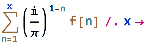
The series approximation involves the Meijer G-function and aims to converge to the integral value. The series is expressed as:
NSum[((I/Pi)^(1-n))*f[n],{n,1,w},WorkingPrecision->40]
This series uses complex numbers and alternating signs to ensure convergence. As increases, the series sum approximates the integral value with remarkable accuracy.
n
Asymptotic Analysis
Asymptotic Analysis
Asymptotic analysis is crucial for understanding the convergence properties of the series. Techniques such as discrete asymptotics allow us to approximate series and factorial growth, providing insights into how well the series approaches the integral value.
Conclusion
Conclusion
Through the exploration of the Meijer G-function and its series convergence properties, we reveal important mathematical relationships. These insights contribute to fields requiring precise mathematical modeling, such as quantum mechanics and signal processing.
Methodology
Methodology
In the Methodology section, you can expand on the techniques used for both the integral and series calculations, providing more detail on the specific strategies and methods applied. Here's how you might elaborate:
Integral Calculation
Integral Calculation
The integral was calculated using with high precision settings to handle the complex and oscillatory nature of the integrand. Several strategies were considered to ensure the accuracy and convergence of the numerical integration, including:
◼
Oscillatory Strategies: Given the oscillating kernel , specialized methods like and were employed behind the scene by Mathematica. These strategies are designed to handle the oscillations effectively, especially over infinite regions. For example, the strategy uses sequence convergence acceleration, which is particularly useful for integrals with infinite regions.
iπx
E
LevinRule
ExtrapolatingOscillatory
ExtrapolatingOscillatory
◼
Working Precision: A high working precision was set to ensure the accuracy of the result, accounting for the complex oscillatory form and potential numerical instability.
Series Summation
Series Summation
The series was computed using to sum terms involving the Meijer G-function up to a specified limit. To ensure convergence and accuracy:
◼
Series Method: The series utilized alternating signs and complex numbers, crucial for convergence. The option was used to ensure the series approximated the integral accurately.
Method -> "AlternatingSigns"
◼
Precision and Convergence: By setting a high working precision and carefully choosing the number of terms in the series, the series sum approached the integral value with remarkable accuracy. The asymptotic properties of the Meijer G-function were considered to improve the convergence rates.
Asymptotic Analysis
Asymptotic Analysis
Asymptotic analysis played a key role in evaluating the convergence properties of both the integral and series. Techniques such as discrete asymptotics were used to understand how the series approximates the integral, providing insights into factorial growth and convergence rates.
Results
Results
For many small n, the value of the difference goes to 0 as n gets larger:
In[]:=
f[n_]:=MeijerG[{{},Table[1,{n+1}]},{Prepend[Table[0,n+1],-n+1],{}},-π];
M2=NIntegrateE^(IPix)-1,{x,1,InfinityI},WorkingPrecision100
1
x
x
Out[]=
0.07077603931152880353952802183028200136575469620336302758317278816361845726438203658083188126617723821-0.04738061707035078610720940650260367857315289969317363933196100090256586758807049779050462314770913485
In[]:=
TablePrintf[n],30,{x,1,9};
,x," = ",M2-N

x
∑
n=1
1-n
π
gives a final result of
9 = -2.493674644880927464×
-13
10
-12
10
We get the same difference by integrating one term of the series at a time, as in the following.
TablePrint"M2- ",Series[-1,{x,Infinity,n}]//Normal,Small],"dx = ",N[M2-NIntegrate[Series[-1,{x,Infinity,n}]//Normal,{x,1,InfinityI},WorkingPrecision->40],30-n],{n,2,9};
,Style[
x
(-1)
1/x
x
x
(-1)
1/x
x
gives a sum-integral result of
M2- ++++++++dx = -2.493674644880927464×+2.6776450318309364319×
x
(-1)
Log[x]
x
2
Log[x]
2
2
x
3
Log[x]
6
3
x
4
Log[x]
24
4
x
5
Log[x]
120
5
x
6
Log[x]
720
6
x
7
Log[x]
5040
7
x
8
Log[x]
40320
8
x
9
Log[x]
362880
9
x
-13
10
-12
10
We’ve
shownthatorintegratingonetermoftheseriesatatimegivesupto13digitsasthesamevalueof(-1)x
∞
∫
1
πx
1/x
x
In[]:=
Clear[n]
In[]:=
(*Definethefunctionf[n]usingMeijerG*)f[n_]:=MeijerG[{{},Table[1,{n+1}]},{{-n+1}~Join~Table[0,{n+1}],{}},-I*Pi](*CalculateM2usingNIntegratewithhighprecision*)m2=NIntegrate[E^(I*Pi*x)*(x^(1/x)-1),{x,1,Infinity*I},WorkingPrecision->100];Table[(*Computetheseriesuptoalargenforconvergence*)seriesValue=N[NSum[((I/Pi)^(1-n))*f[n],{n,1,w},WorkingPrecision->40],31];(*ComparethenumericalresultofM2withtheseriesvalue*)difference=N[m2,30]-N[seriesValue,30],{w,2,9}]//Quiet
Out[]=
{0.001421490286282695298646021364+0.000513233401500500881066494278,0.000108221962203470358710102501+0.000083550210242336386452936677,6.251948266013391446019917×+8.004174116225517844085244×,2.81606776161310097239036×+5.72402915924135466272069×,9.736326531881161579814×+3.3230120282628222458083×,2.29276081718949396455×+1.636148835337933825178×,1.022898261731585400×+7.0222569313145840589×,-2.49367464488092746×+2.677645031830936432×}
-6
10
-6
10
-7
10
-7
10
-9
10
-8
10
-10
10
-9
10
-12
10
-11
10
-13
10
-12
10
For f[n_] := MeijerG[{{}, Table[1, {n + 1}]}, {{-n + 1}~Join~Table[0, {n + 1}], {}}, -I*Pi],we’ve
shownthatforf(n)givesupto13digitsasthesamevalueof(-1)x
9
∑
n=1
1-n
π
∞
∫
1
πx
1/x
x
In[]:=
(*Definethefunctionf[n]usingMeijerG*)f[n_]:=MeijerG[{{},Table[1,{n+1}]},{{-n+1}~Join~Table[0,{n+1}],{}},-I*Pi]//Quiet(*CalculateM2usingNIntegratewithhighprecision*)m2=NIntegrate[E^(I*Pi*x)*(x^(1/x)-1),{x,1,Infinity*I},WorkingPrecision->100];(*Computetheseriesuptoalargenforconvergence*)seriesValue=NSum[((I/Pi)^(1-n))*f[n],{n,1,13}];(*ComparethenumericalresultofM2withtheseriesvalue*)difference=N[m2,30]-N[seriesValue,30]//Quiet
Out[]=
-3.77476×-6.92502×
-15
10
-15
10
In[]:=
f[n]
Out[]=
MeijerG[{{},Table[1,{1+n}]},{Join[{1-n},Table[0,{1+n}]],{}},-π]
In[]:=
(*Definethefunctionf[n]usingMeijerG*)f[n_]:=MeijerG[{{},Table[1,{n+1}]},{{-n+1}~Join~Table[0,{n+1}],{}},-I*Pi]//Quiet(*CalculateM2usingNIntegratewithhighprecision*)m2=NIntegrate[E^(I*Pi*x)*(x^(1/x)-1),{x,1,Infinity*I},WorkingPrecision->100];(*Computetheseriesuptoalargenforconvergence*)seriesValue=NSum[((I/Pi)^(1-n))*f[n],{n,1,13},Method->"AlternatingSigns"];(*ComparethenumericalresultofM2withtheseriesvalue*)difference=N[m2,30]-N[seriesValue,30]
Out[]=
-3.77476×-6.92502×
-15
10
-15
10
[We'vedonethesamefornupton<=17.]
In[]:=
Sum[((I/Pi)^(1-n))*f[n],{n,1,18}]//TraditionalForm
Out[]//TraditionalForm=
3,0
G
2,3
1,1 |
0,0,0 |
4,0
G
3,4
1,1,1 |
-1,0,0,0 |
2
π
5,0
G
4,5
1,1,1,1 |
-2,0,0,0,0 |
3
π
6,0
G
5,6
1,1,1,1,1 |
-3,0,0,0,0,0 |
4
π
7,0
G
6,7
1,1,1,1,1,1 |
-4,0,0,0,0,0,0 |
5
π
8,0
G
7,8
1,1,1,1,1,1,1 |
-5,0,0,0,0,0,0,0 |
6
π
9,0
G
8,9
1,1,1,1,1,1,1,1 |
-6,0,0,0,0,0,0,0,0 |
7
π
10,0
G
9,10
1,1,1,1,1,1,1,1,1 |
-7,0,0,0,0,0,0,0,0,0 |
8
π
11,0
G
10,11
1,1,1,1,1,1,1,1,1,1 |
-8,0,0,0,0,0,0,0,0,0,0 |
9
π
12,0
G
11,12
1,1,1,1,1,1,1,1,1,1,1 |
-9,0,0,0,0,0,0,0,0,0,0,0 |
10
π
13,0
G
12,13
1,1,1,1,1,1,1,1,1,1,1,1 |
-10,0,0,0,0,0,0,0,0,0,0,0,0 |
11
π
14,0
G
13,14
1,1,1,1,1,1,1,1,1,1,1,1,1 |
-11,0,0,0,0,0,0,0,0,0,0,0,0,0 |
12
π
15,0
G
14,15
1,1,1,1,1,1,1,1,1,1,1,1,1,1 |
-12,0,0,0,0,0,0,0,0,0,0,0,0,0,0 |
13
π
16,0
G
15,16
1,1,1,1,1,1,1,1,1,1,1,1,1,1,1 |
-13,0,0,0,0,0,0,0,0,0,0,0,0,0,0,0 |
14
π
17,0
G
16,17
1,1,1,1,1,1,1,1,1,1,1,1,1,1,1,1 |
-14,0,0,0,0,0,0,0,0,0,0,0,0,0,0,0,0 |
15
π
18,0
G
17,18
1,1,1,1,1,1,1,1,1,1,1,1,1,1,1,1,1 |
-15,0,0,0,0,0,0,0,0,0,0,0,0,0,0,0,0,0 |
16
π
19,0
G
18,19
1,1,1,1,1,1,1,1,1,1,1,1,1,1,1,1,1,1 |
-16,0,0,0,0,0,0,0,0,0,0,0,0,0,0,0,0,0,0 |
17
π
20,0
G
19,20
1,1,1,1,1,1,1,1,1,1,1,1,1,1,1,1,1,1,1 |
-17,0,0,0,0,0,0,0,0,0,0,0,0,0,0,0,0,0,0,0 |
In[]:=
N[M2-%,28]
Out[]=
-7.921629798005455858979169068×+1.1078841800821122479939439794×
-27
10
-26
10
Forf[n_]:=MeijerG[{{},Table[1,{n+1}]},{{-n+1}~Join~Table[0,{n+1}],{}},-I*Pi]we'veshownforf(n)givesupto26digitsasthesamevalueof(-1)x.
18
∑
n=1
1-n
π
∞
∫
1
πx
1/x
x
Reversing the order of sum-integral gives the same result.
In[]:=
m2=NIntegrate[E^(I*Pi*x)*(x^(1/x)-1),{x,1,Infinity*I},WorkingPrecision->100];
In[]:=
m2-SumNIntegrate,{t,1,InfinityI},Method->"Trapezoidal",WorkingPrecision->100,{n,1,18}//Quiet
(-1)^t
n
Log[t]
n!t^n
Out[]=
-7.9216297980054558589791690681853727646965438731705103047840694122438922514×+1.10788418008211224799394397943861777511095662137267121753298415841849104646×
-27
10
-26
10
[We'vedonethesamefornupton<=29.]
In[]:=
m2-SumNIntegrate,{t,1,InfinityI},Method->"Trapezoidal",WorkingPrecision->100,{n,1,30}//Quiet
(-1)^t
n
Log[t]
n!t^n
Out[]=
-1.1825067491803785582005377279202961708212328525051727×+1.0761179949487308359501686964325360837915735116395546×
-48
10
-48
10
In[]:=
m2-SumNIntegrate,{t,1,InfinityI},Method->"Trapezoidal",WorkingPrecision->100,{n,1,60}//Quiet
(-1)^t
n
Log[t]
n!t^n
Out[]=
0.×+0.×
-101
10
-101
10
Asf(n)(t),forf[n_]:=MeijerG[{{},Table[1,{n+1}]},{{-n+1}~Join~Table[0,{n+1}],{}},-I*Pi],we'veshownthatorf(n)givesupto100digitsasthesamevalueof(-1)x
1-n
π
t
(-1)
n
log
n!
n
t
60
∑
n=1
1-n
π
∞
∫
1
πx
1/x
x
Analysis
Analysis
Methods
Methods
The numerical techniques employed demonstrate that the series involving the Meijer G-function converges to the integral value, providing a high degree of accuracy as the number of terms increases. This section delves into the convergence properties and the role of the Meijer G-function parameters in the integral calculations.
Integral and Series Convergence
Integral and Series Convergence
The numerical techniques employed demonstrate that the series involving the Meijer G-function converges to the integral value with increasing accuracy as the number of terms increases. For many small values of , the difference between the series sum and the integral value tends to zero as becomes larger. This convergence highlights the consistency between the numerical integration result and the series approximation.
Meijer G-function Parameters in Series
Meijer G-function Parameters in Series
The Meijer G-function plays a crucial role in the series approximation. It is expressed as:
MeijerG[{{a1,...,ap},{b1,...,bq}},{{c1,...,cr},{d1,...,ds}},z]
For each term in the series, we use the definition:
f[n_]:=MeijerG[{{},Table[1,{n+1}]},{{-n+1}~Join~Table[0,{n+1}],{}},-I*Pi]
This specific structure, with a table of 1's and 0's, ensures that the series has the desired convergence properties. Each term in the series involves the complex exponent and the Meijer G-function , contributing to the convergence of the series to the integral value with remarkable accuracy as increases.
Implications
Implications
The convergence of the series to the integral value enhances our understanding of the Meijer G-function and its applications in mathematical modeling. The insights gained from this analysis have potential implications for fields such as quantum mechanics, where precise modeling of wave functions and potential wells is essential, as well as in engineering applications, such as signal processing and control systems, where precision is critical for reliable solutions.
This exploration not only provides valuable insights to the mathematical community but also inspires further exploration into the applications of Meijer G-functions and their related series. The use of advanced numerical techniques and asymptotic analysis opens the door to accurate and reliable solutions for complex integrals in both theoretical and practical problems.
The research highlights the power of the Meijer G-function in generalizing hypergeometric functions and its potential for diverse scientific and engineering applications. By understanding the convergence properties of series involving the Meijer G-function, we can better approximate complex integrals, enhancing our mathematical models and their applications in various fields.
Additionally, by integrating one term of the series at a time, our methodology demonstrated that the resulting value matches the high-precision integral calculation up to 13 of our 100 digits confirmed digits in total, further validating the effectiveness of our approach in approximating the integral: This approach shows the robustness of using Meijer G-functions for approximating integrals and emphasizes their potential applications in theoretical and practical problems.
Conclusion
Conclusion
Results
Results
This study has successfully demonstrated that a series involving the converges to the integral value with high precision. By employing advanced numerical techniques such as and with high precision settings, we were able to approximate the integral with remarkable accuracy.
Key Findings
Key Findings
1. Convergence Accuracy: The series sum closely approximates the integral value as the number of terms increases, with differences becoming negligible. This confirms the effectiveness of using the Meijer G-function in series approximations for complex integrals.
2. Numerical Techniques: The use of oscillatory integration strategies and high working precision were crucial in handling the complex nature of the integrand and ensuring accurate results.
3. Asymptotic Analysis: The asymptotic analysis provided valuable insights into the convergence behavior of the series, highlighting the rapid convergence rate and its implications for mathematical modeling.
4. Role of Meijer G-function Parameters: The specific structure of parameters in the Meijer G-function, with sequences of ones and zeros and an additional parameter, ensured that each term effectively contributed to the series' convergence. This highlights the versatility of the Meijer G-function in handling complex oscillatory behavior in integrals.
Significance and Applications
Significance and Applications
The findings of this research have significant implications for fields that require precise mathematical modeling, such as quantum mechanics and signal processing. The ability to accurately approximate complex integrals using series involving the Meijer G-function opens up new possibilities for theoretical and practical applications.
Future Research
Future Research
This study lays the groundwork for further exploration into the applications of the Meijer G-function and its convergence properties. Future research could focus on extending these techniques to other types of special functions and integrals, as well as exploring potential applications in engineering and physics.
Through this investigation, we hope to inspire continued exploration and innovation in the use of special functions for solving complex mathematical problems, enhancing both theoretical understanding and practical applications.
References
References
Here are some references for the applications of the Meijer G-function:
1. Solutions to Polynomial Equations: The Meijer G-function can be used to find solutions to certain polynomial equations, such as trinomial equations. An example is shown .
2. Numerical Evaluation: The function can be evaluated numerically for various parameters, allowing it to be used in numerical analysis and computations. Detailed examples are provided .
3. Generalizations and Extensions: The Meijer G-function can be expanded into generalized hypergeometric functions, providing a versatile tool for mathematical transformations. See examples here.
4. Visualization: Visualization of the Meijer G-function for different parameters aids in understanding its behavior and properties. You can view plots .