Introduction:
Introduction:
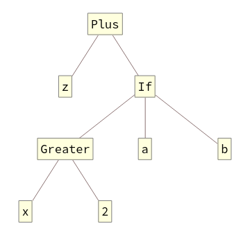
In the Wolfram Language, there are many built-in functions to help visualize one’s code. For example, if someone wanted to see the structure of their code, they could use the TreeForm command:
TreeForm[If[x>2,a,b]+f/@z]
Out[]//TreeForm=
Or, they could use something like the Trace Command:
Trace@(Sin[Pi]^2+Cos[Pi]^2+1)
Out[]=
{{{Sin[π],0},,0},{{Cos[π],-1},,1},0+1+1,2}
2
0
2
(-1)
The issue with these visualization functions is that they’re a bit too specific, which makes it difficult to intuitively understand what the program is doing. There are also some functions that don’t show up in TreeForm; Map, for example, was one of these functions. There is a function called NetGraph that will give a general graph of how information flows in a neural network, but at the moment NetGraph only works for neural networks. The BlockDiagram function tries to combine the ideas of TreeForm and NetGraph to provide a more general view of the flow of a program. The goal of this post is to provide an explanation for how the BlockDiagram function works.
The BlockForm Helper Function
The BlockForm Helper Function
The heart of the BlockDiagram function is the BlockForm helper function. The BlockForm function consists of three parts: creating the adjacency list for the graph of the function, graphing the function, and then calling BlockForm again on each of the vertices. Here is what the BlockForm definition looks like for the If function.
In[]:=
BlockForm[inputCode_If,OptionsPattern[]]:=With[{code=HoldForm[inputCode]},Module[{adjacencylist={{1,1}{1,2}},edgestyle={{1,1}{1,2}Darker@Darker@Green},edgelabels={{1,1}{1,2}Framed["True",BackgroundLighter@LightBlue]}},With[{positions=Position[code,_[___]|_?AtomQ,2,HeadsFalse]},If[MemberQ[positions,{1,3}],AppendTo[adjacencylist,{1,1}{1,3}];AppendTo[edgestyle,{1,1}{1,3}Darker@Darker@Red];AppendTo[edgelabels,{1,1}{1,3}Framed["False",BackgroundLighter@LightBlue]]];If[MemberQ[positions,{1,4}],AppendTo[adjacencylist,{1,1}{1,4}];AppendTo[edgelabels,{1,1}{1,4}Framed["Neither",BackgroundLighter@LightBlue]]];TreePlot[Graph[adjacencylist,VertexShapeFunction(Which[#2{1,1},conditionalvertexfunction[code,OptionValue["DynamicDisplayFunction"],.15][#1,#2,#3],True,dvsf[code,OptionValue["DynamicDisplayFunction"]][#1,#2,#3]]&),EdgeStyleedgestyle,EdgeLabelsedgelabels,EdgeShapeFunction"DashedLine",ImageSizeOptionValue["ImageSize"],PerformanceGoal"Quality"],Left]]]]
The adjacency list defined in this graph may look somewhat odd because at a first glance it doesn’t appear to have anything to do with an If statement. However, what the adjacency list represents is the positions of the parts of an If statement. Here’s an example. If I want to get the position of the condition in the If statement, I can write:
The adjacency list defined in this graph may look somewhat odd because at a first glance it doesn’t appear to have anything to do with an If statement. However, what the adjacency list represents is the positions of the parts of an If statement. Here’s an example. If I want to get the position of the condition in the If statement, I can write:
Position[If[x1,a,b],x1]
Out[]=
{{1}}
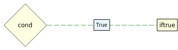
Now, this probably leads the reader to two questions: how do I know how the positions connect and why is the position for our condition in the adjacency list labeled {1,1} instead of just {1}? Let’s first look at the first question. In general, there are three possible cases for an If statement. The first is when the If statement has two arguments: a condition to check and code to run if the condition is true. It has the form If[cond,iftrue].
Out[]=
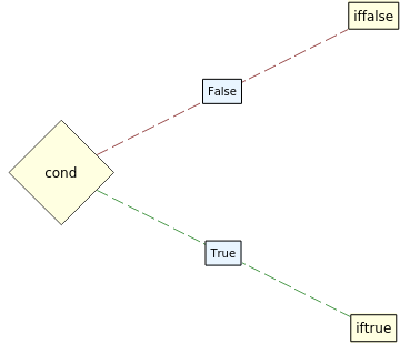
The second case is when there’s a condition, code to run if the condition is true, and code to run if the condition is false. It has the form If[cond,iftrue,iffalse].
Out[]=
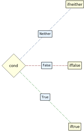
And the third case is when there’s a condition, code to run if the condition is true, code to run if the condition is false, and code to run if the condition is neither true nor false. It has the form If[cond,iftrue,iffalse,ifneither].
Out[]=
For all these cases, we can see that the first argument (the condition) connects to the second, third, and fourth argument of the If statement. So, when we draw our adjacency list, we will have position {1} connect to position {2}, and then it will check whether it should connect {1} to {3} or {1} to {4}. A lot of functions have a fixed pattern of data flow like this, so to create the BlockForm for a function, one just needs to know the pattern that the arguments follow.
The second question is “why do the positions have an extra 1 prepended to them?”. The reason why is because the input is wrapped in a function called HoldForm, which adds an extra level to our function when taking the position of it. For example, if we compare taking the condition of an if statement and taking the condition of an if statement with HoldForm we get:
The second question is “why do the positions have an extra 1 prepended to them?”. The reason why is because the input is wrapped in a function called HoldForm, which adds an extra level to our function when taking the position of it. For example, if we compare taking the condition of an if statement and taking the condition of an if statement with HoldForm we get:
Position[If[x1,a,b],x1]
Out[]=
{{1}}
Position[HoldForm@If[x1,a,b],x1]
Out[]=
{{1,1}}
A quick follow-up question would be “why does the function wrap the input in a HoldForm function”? The reasons why are because we don’t want our input code to ever evaluate in our diagram (so we can model programs that involve functions like Set or mathematical expressions like Sin[Pi], which would normally evaluate otherwise) and because HoldForm does not change the appearance of the code like Hold does. Here is a quick visual comparison of Hold and HoldForm.
Hold@Sin[Pi]
Out[]=
Hold[Sin[π]]
HoldForm@Sin[Pi]
Out[]=
Sin[π]
A lot of the quirky looking code (the adjacency lists having a prepended 1 to the vertices, HoldForm being in the code everywhere, etc.) can be explained by the fact that the input needs to be held at all times, and the code must be changed to accommodate for this fact. That is basically how the first step of BlockForm works. The second step is pretty simple. It graphs the adjacency list using functions like Graph, TreePlot, and LayeredGraphPlot, and it styles them using the EdgeLabels, EdgeStyle, and EdgeShapeFunction options. The third step is to call the BlockForm function on each of the vertices. The program does this by having a Vertex Shape Function change the shape of each vertex to the BlockForm of the code it contains. Here is a visual example. First, we see the result of the first iteration of BlockForm.
BlockForm[If[x2,Nodify@Print[x],Nodify@Print[y]]]
Out[]=
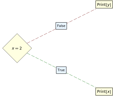
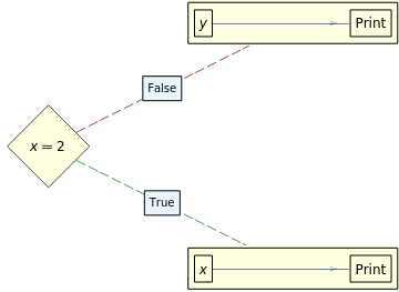
The result of running BlockForm on each vertex turns them into their respective Block Form. Note that x==2 does not change because it is already reduced to its Block Form.
BlockForm[If[x2,Print[x],Print[y]]]
Out[]=
One thing to note about the above line of code is that the function that only evaluates BlockForm once involves a function called Nodify. Nodify is a wrapper function that tells the program to stop calling BlockForm on this vertex and just output its argument. A weird thing to note about Nodify is that it’s not defined anywhere, but because BlockForm handles input based on expression heads, one can use Nodify with the expression handler as if it were a function. Here is the definition of the Nodify handler in BlockForm.
BlockForm[inputCode_Nodify,OptionsPattern[]]:=If[OptionValue[SecondaryIteration],Extract[HoldForm@inputCode,{1,1},HoldForm],Graph[{{1,1}},{},VertexShapeFunctiondvsf[HoldForm@inputCode,OptionValue["DynamicDisplayFunction"]],ImageSizeAutomatic,PerformanceGoal"Quality"]]
Putting It All Together (Using DynamicModule and the dvsf Helper Function)
Putting It All Together (Using DynamicModule and the dvsf Helper Function)
To combat the fact that a graph may become too large to display correctly, the BlockDiagram function has some elements of interactivity where if the user clicks on a vertex, it will show a zoomed in version of the graph inside the vertex. Here is one example of an interactive graph produced by the BlockDiagram function. Please note that because BlockDiagram uses the DynamicModule function, it must be re-run in order to maintain the interactive graph; because code can’t be executed within a blog post, the output of BlockDiagram has been replaced with pictures to remain consistent.
In[]:=
BlockDiagram[If[x>2,a,b]+f/@z]
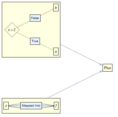
The BlockDiagram function uses a DynamicModule that stores a list of current and previously displayed graphs. It will always display the first graph inside the list. When a user clicks a vertex, the graph of the vertex is prepended to the list of graphs, and because it dynamically always shows the first element of the list, it will show the graph of the vertex. In addition to the ability to zoom in, one can also zoom out by clicking the Back («) button. It will remove the first element (the graph of the vertex) from the list and will display the original graph again (because it goes back to being the first element). It basically behaves like a Stack. Below is the code for the BlockDiagram function.
BlockDiagram[inputCode_]:=DynamicModule[{blockdiagramdisplay},Dynamic[Labeled[First[blockdiagramdisplay],If[Echo@TrueQ[Length@blockdiagramdisplay>1],Button[Style["«",20,Bold],blockdiagramdisplay=Rest@blockdiagramdisplay],""],Left],Initialization(blockdiagramdisplay={BlockForm[inputCode,"DynamicDisplayFunction"(PrependTo[blockdiagramdisplay,#]&)]})]]
One final thing I want to discuss is the Default Vertex Shape Function (dvsf) function. The dvsf is not only what formats the vertices (by calling BlockForm on them), but it is also what connects the recursive structure of BlockForm to the dynamic structure of BlockDiagram. The dvsf contains a callback function to the BlockDiagram so that whenever a vertex is clicked, the graph of that vertex is prepended to the list of graphs stored in the DynamicModule in the BlockDiagram function. The code for the dvsf can be found below.
dvsf[code_,buttonf_]:=(With[{expr=Extract[code,#2,HoldForm]},{Black,With[{bf=BlockForm[expr,SecondaryIterationTrue,"DynamicDisplayFunction"buttonf]},Inset[Button[Framed[BlockForm[expr,SecondaryIterationTrue,"DynamicDisplayFunction"buttonf,"ImageSize"Tiny]],buttonf@bf,AppearanceNone],#1,BackgroundRGBColor[1,1,0.88]]]}]&)
Conclusion
Conclusion
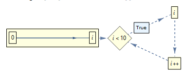
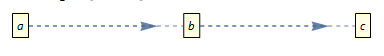
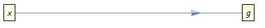
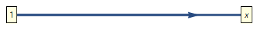
To reiterate, the BlockDiagram function attempts to create a more intuitive diagram of a program. It does this by recursively making an interactive graph of each level of a function. Currently, it is still only a proof of concept, but in the future it could become a better way to visualize code in the Wolfram language. Here are a few more examples to play around with, just to show what the code can do. To better understand the graphs, the dashed lines mean procedural steps, the thick arrows represent assignment, and the thin arrows mean that the code is an argument of what it points to.
In[]:=
BlockDiagram[For[i=0,i<10,i++,i]]
In[]:=
BlockDiagram[a;b;c]
In[]:=
BlockDiagram[g[x]]
BlockDiagram[x=1]
Source Code At The Time
Source Code At The Time