This is a part 2 to my previous post which had provided a means to tinker with our thought processes and manipulate them with the wolfram language. It was a purely conceptual idea limited due to the lack of electronics which would be interfacing with the brain. Recently, I have been experimenting with the OpenBCI kit in order to better understand the language which the brain speaks. The elementary problems I will be solving in this post is to identify stimuli like jaw clench or eye blink from the electroencephalographic(EEG) readings extracted from the outside of the brain. This will require a cocktail of signal processing, machine learning and brain computer interface.
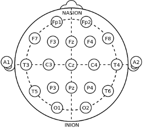
In order to record useful EEG data, I will be using the 10-20 system which is an internationally recognized method to describe and apply the location of scalp electrodes for standardization of readings.
Our brains are always at work! Biochemistry exchanges between cells produce small electrical activity when the neurons communicate among themselves. A single electric signal from neuron to neuron is not recordable but when millions of neurons synchronize, the electric field generated can be measured from the scalp.These signals are transmitted through tissue, bone, and hair before it is recorded, and by then its amplitude is very noisy.
This can be compared to attaching sensors outside a factory in order to understand what’s going on inside. The machines inside the factory would produce thermal and vibrational energy, which would transmit across the walls to the sensors, revealing information about the machine operations and hence the workings of the factory .
An “artifact ” is any component of the EEG signal that is not directly produced by the human brain activity. The ability to recognize these artifacts is the first step in removing them. In this study I will be trying to identify ocular artifacts (eye blink) or muscular artifacts(jaw clench) using a convolutional neural network. The reason behind the choice of this neural net architecture will be discussed later.
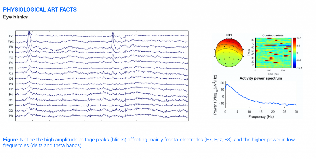
The eye can be electrically modelled as a magnetic dipole and it distorts the electric field in the region when it moves. Blinking produces a Dirac-delta on the EEG-signal, reaching about 100-200 microvolts. The signal is strongest at the frontal part of the head, corresponding to F7, F8, Fp1 and Fp2 channels in the 10-20 system.
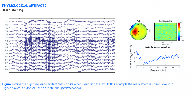
Muscle produces electrical activity when they are contracted called electromyography. For example, clenching the jaw can result in a high frequency signal whose amplitudes correlates with the strength of the muscle contraction. The signal is strongest at the F3, C3, F4 and C4 channels corresponding to the 10-20 system.
Some other interesting physiological artifacts include cardiac activity which produce a rhythmic pattern as well as, perspiration and respiration which produce low frequency shallow waves on top of the EEG signal. Apart from these, other sources of non-psychological artifacts come from electrode pop, cable movement and incorrect reference placement.
Some other interesting physiological artifacts include cardiac activity which produce a rhythmic pattern as well as, perspiration and respiration which produce low frequency shallow waves on top of the EEG signal. Apart from these, other sources of non-psychological artifacts come from electrode pop, cable movement and incorrect reference placement.
From a computational point of view, the raw EEG signal is simply a discrete time multivariate(i.e with multiple dimensions) time dimensions. The dataset consists of 14-channel(or dimensions) EEG data sampled at 128Hz i.e 128 samples per second for 6 minutes.
The first 30 seconds is baseline calibration data, with the initial 15 seconds recorded with eyes open and the remaining 15 with eyes closed. After this, instances of eye blink and jaw clench artifacts occur for the remaining time. These time instance of these artifacts are seperatley recorded in order to extract the correct EEG data.
A windows size of 0.5 seconds is assumed (0.2 seconds before the marker and 0.3 seconds after the marker). Additionally, only the F3 and F4 channels are considered as they accurately detect eye blink as well as jaw clench.
Data Cleaning
Data Cleaning
The first step is to take EEG data from channels F3 and F4 to extract the required markers for jaw clench and eye blink. As the window size is chosen to be 0.5 s (0.2s before the marker and 0.3s after the marker), the data will be sampled to 0.5 s or 64 samples (128/2 ).We can also sample the data at 0.1 s(sample size 128/10=12.8) in order to select the window size of 0.2 before and 0.3 later. By approximating 12.8 to 13, we are reducing the accuracy by 1.5%. Different sample sizes with varying size can be further tested to boost bias of the neural network.
Out[]=
The number of samples should be equal to 128 samples *6 min* 60s = 46080
Length[af3data]
Out[]=
46066
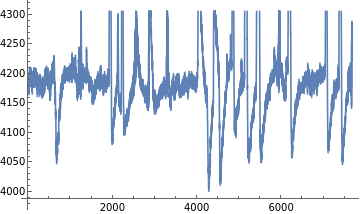
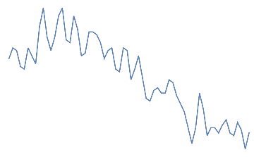
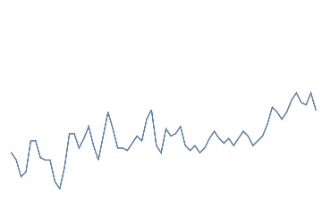
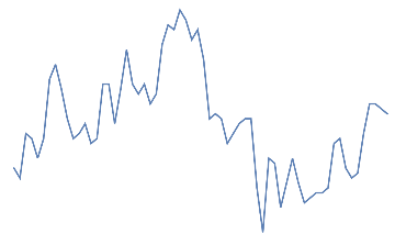
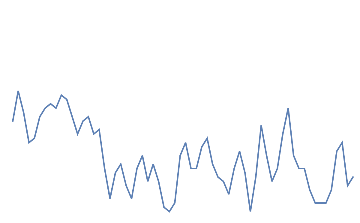
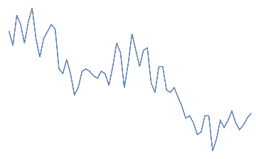
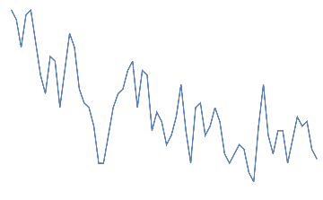
The open eye and close eye last for the first 30s as well as a 5s gap in-between, corresponding to 4480 samples.
In[]:=
ListLinePlot[Take[af3data,4480],AxesFalse]
Out[]=
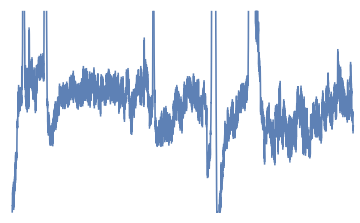
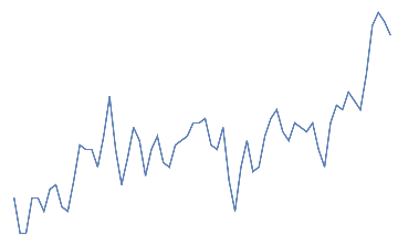
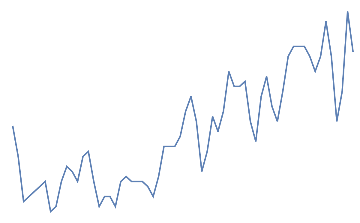
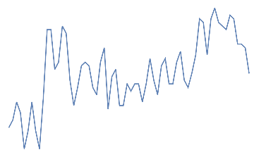
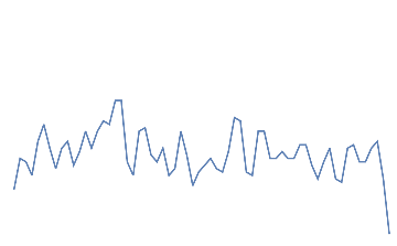
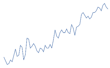
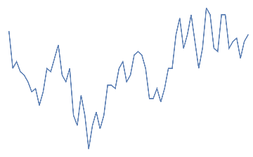
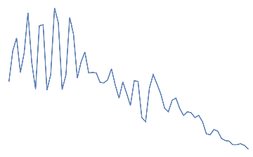
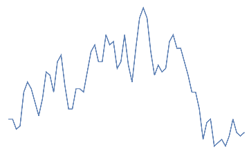
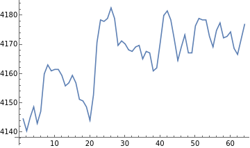
Following is the plot(F3) for 1 minute after the baseline data.
In[]:=
ListLinePlot[Take[af3data,{4481,12160}],AxesTrue]
Out[]=
This same procedure is repeated for the F4 data.
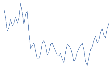
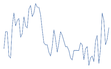
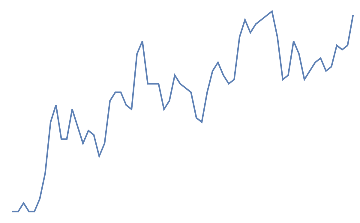
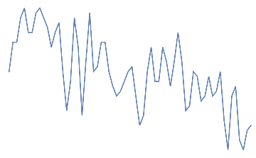
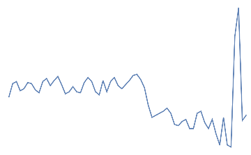
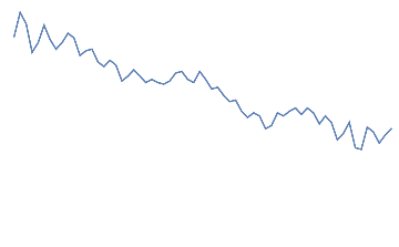
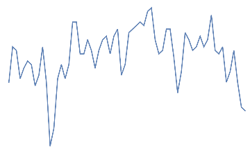
Applying bipolar EEG(F3-F4) and a gamma band pass filter to remove noise and get a more localized picture.
eegdata=BandpassFilter[af3data-af4data,{31,40}];ListLinePlot[eegdata]
Out[]=
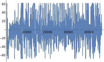
The bandpass filter is taken in the 31-40 Hz(or gamma) frequency range as this corresponds to conscious or perceptive thinking.
Additionally, common average or reference electrode standardization technique can be used to optimize the data. From now onwards, the bipolar EEG data will be considered.
Next, the EEG data is manually compared with the instances of the artefacts recorded. After thorough inspection, the following order of events is noted.
Eyes Open (15.1s) ->5s->Eyes Close(15s)->11.3s->blink->2,2s->blink->3.2s->......->jaw->3s->blink->3.6s->blink->2.9s->jaw->9.5s->jaw->8s
The total time duration for all the complete set of actions is 352s whereas the time duration of the experiment is 360s. This might be due to the limitations of the hardware setup or because there is an 8s idle time after the last jaw clench instance.This data is sampled at 0.1s and hence, the time intervals are multiplied by 10(deci-second). For each 0.1s, we will recieve approximately 13 data points. In total, there are 44 instances of eye blink and 38 instances of jaw clench.
The window size of 0.5s(0.2s before and 0.3s later) would correspond to 64 readings(26 before the instance and 38 after the instance). 26 has been rounded up from 25.8 and 38 has been rounded down from 38.4.
Imported artifact readings(taken in deciseconds):
In[]:=
Sort@Join[#"eye blink"&/@Flatten[Take[artefacts,44]],#"jawclench"&/@Flatten[Take[artefacts,{45,82}]]]
Out[]=
{464.eye blink,486.eye blink,518.jawclench,537.jawclench,567.jawclench,627.eye blink,657.eye blink,690.eye blink,713.jawclench,737.eye blink,776.jawclench,799.eye blink,868.eye blink,894.eye blink,916.jawclench,951.jawclench,982.eye blink,1012.jawclench,1040.eye blink,1070.eye blink,1099.jawclench,1153.jawclench,1206.jawclench,1244.eye blink,1274.eye blink,1324.eye blink,1355.jawclench,1397.jawclench,1425.jawclench,1468.eye blink,1508.eye blink,1546.eye blink,1571.jawclench,1616.eye blink,1652.eye blink,1687.jawclench,1735.jawclench,1771.eye blink,1805.jawclench,1844.jawclench,1878.eye blink,1914.jawclench,1947.jawclench,1994.eye blink,2036.eye blink,2074.eye blink,2109.eye blink,2131.jawclench,2170.jawclench,2206.jawclench,2235.eye blink,2281.eye blink,2322.eye blink,2351.jawclench,2398.jawclench,2449.eye blink,2486.eye blink,2532.eye blink,2602.jawclench,2632.eye blink,2663.eye blink,2702.eye blink,2730.jawclench,2777.jawclench,2819.eye blink,2857.jawclench,2911.jawclench,2964.eye blink,2996.eye blink,3026.eye blink,3047.jawclench,3080.jawclench,3123.eye blink,3167.eye blink,3213.jawclench,3271.jawclench,3305.eye blink,3335.jawclench,3365.eye blink,3401.eye blink,3430.jawclench,3525.jawclench}
Preparing the training and testing data set
Preparing the training and testing data set
The dataset is extracted and labelled for supervise learning.
keyval[x_] is a function that can locate the artifact instance value given and extract the EEG information in the specified window size according to the specification(0.2 second before and 0.3 second later). It is essentially a link between the EEG time counter and channel.
keyval[x_] is a function that can locate the artifact instance value given and extract the EEG information in the specified window size according to the specification(0.2 second before and 0.3 second later). It is essentially a link between the EEG time counter and channel.
In[]:=
keyval[x_]:=Association[Flatten[{#eegdata[[#]]}&/@Range@Length@Drop[Flatten[af3data],1]]][#]&/@Flatten@Flatten@{Round[x*12.8]+#}&/@Sort@Join[Minus[Range[26]],Range[38]]Length@keyval[56.8]
Out[]=
64
An additional dataset corresponding to “neither jaw clench or eye blink” has been taken from initial 30s as a buffer.
In[]:=
nothingdata=Rasterize[ListLinePlot[#,AxesFalse]]"nothing"&/@Take[Partition[eegdata,64],{10,20}]
Out[]=
nothing,
nothing,
nothing,
nothing,
nothing,
nothing,
nothing,
nothing,
nothing,
nothing,
nothing
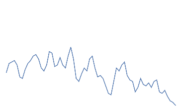
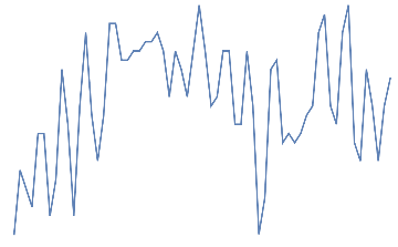
Following is the EEG response for 10 eye blinks. This should be a quick change with high amplitude in the electrodes of the frontal area.
Out[]=
eye blink,
eye blink,
eye blink,
eye blink,
eye blink,
eye blink,
eye blink,
eye blink,
eye blink,
eye blink
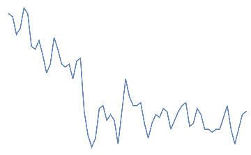
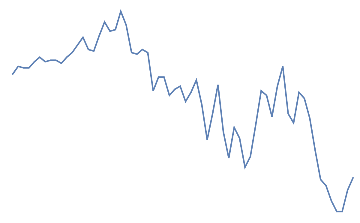
Following is the EEG response for 10 jaw clenches. This should be a high frequency that overlaps the EEG signal.
Out[]=
jaw clench,
jaw clench,
jaw clench,
jaw clench,
jaw clench,
jaw clench,
jaw clench,
jaw clench,
jaw clench,
jaw clench
Next we shuffle all our data together (93 samples), extracting 80%(74) for the training and 20%(19 samples) for the testing.
In[]:=
alldata=BlockRandom[RandomSample@Join[nothingdata,blinkdata,jawdata]];
In[]:=
traindata=Take[alldata,74];
In[]:=
testdata=Keys@Take[alldata,19];
Finding the different classes:
In[]:=
classes=Union@Values[traindata]
Out[]=
{eye blink,jaw clench,nothing}
Machine Learning Architecture
Machine Learning Architecture
The structure of the neural network is inspired by the “LeNet trained on MNIST data”. The thinking is that an MNIST classifier identifies handwriting data which is essentially a specific type of curve. Similarly, the instances in our EEG data are continuous curves.
The EEG curve for a specific artifact like jaw clench are similar, just like all the handwriting data for the number 3 are similar.
The EEG curve for a specific artifact like jaw clench are similar, just like all the handwriting data for the number 3 are similar.
jawclench,
3
In[]:=
myEncoder=NetEncoder[{"Image",{28,28}}];myDecoder=NetDecoder[{"Class",classes}];mynet=NetChain[{ConvolutionLayer[20,5],ElementwiseLayer[Ramp],PoolingLayer[2,2],ConvolutionLayer[50,5],ElementwiseLayer[Ramp],PoolingLayer[2,2],FlattenLayer[],LinearLayer[500],ElementwiseLayer[Ramp],LinearLayer[3],SoftmaxLayer[]},"Input"myEncoder,"Output"myDecoder]
Out[]=
NetChain

Training of the network
In[]:=
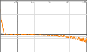
results=NetTrain[mynet,traindata,All,MaxTrainingRounds100]trained=results["TrainedNet"]
Out[]=
Out[]=
NetChain

The loss of the neural net is 0.729 and the error is 32%.
Future Plan
Future Plan
Some of the future plans of the project include:
1
.To create neural net architecture(RNN, LDA) to identify all kinds of artifacts. Applications include Amazon Alexa integration, smart home automation, medical devices, communication, and VR/AR integration.
2
.This exercise is purely based on reading information and interpreting it. Next, I would like to explore writing data into the brain via implant so I can implement the architecture from my previous post.
3
.Improve the efficiency of the neural net by applying better filtering techniques to the data such as CSP(Common Spatial Pattern) and extraction techniques such as principle component analysis.
The Wolfram language is built like a cathedral, “carefully crafted by individual wizards or small band of mages working in splendid isolation”. Whereas, other languages seem “to resemble a great babbling bazaar of different agendas and approaches”. Although the later has several advantages, it disregards security and uniformity which are very important criteria for brain machine interface. Never the less, I believe that human thoughts are more functional than object oriented.
I believe because of the above reasons, the Wolfram language will be the gateway between human and computational thinking for all future brain machine interface devices. Let me know what you think in the comments below!