Abstract
Abstract
This project designs a series of procedures to draw a character on the street map. Given a character, a rotation angle, and a region of interest within a small radius, the output will be a road tour one can walk trough. Based on graph theory, we designed methods to construct a map graph and a character graph. A map graph carries the geo-positional data of street nodes within region of interest; a character map carries the connective relationship between selective pixels on the character map. A portion of map graph will be matched with the character graph in order to generate a new graph that shares the collective properties of the previous two. The FindPostmanTour and FindShortestPath functions takes in the new graph and generate a road tour. One can follow the navigation of the tour such that the trace will be a one-line drawing of the desired character.
Section 1 Extract the Street Map Data
Section 1 Extract the Street Map Data
Given a region, say one centered at New York University, Manhattan within 1 mile radius, I walk around and trace my walk. In which roads, which directions I should walk, such that my trace forms in the shape of a character “A”? As well as in the shortest total distances?
Preliminary Setup
Preliminary Setup
To find out the answer, let’s define some key variables we’ve already know. Take the main campus at New York University as an example. Specify 1 mile at the radius centered at origin that covers our region of interest. Note that a larger radius will result a larger geographical dataset, thus require longer cell evaluation time. Manhattan is a city having crowd roads data, so we might specify a small radius in order to balance the data retrieving time.
Define a origin, a radius centered at origin that covers our region of interest, a character we would like to draw, and a rotation angle at which our final tour rotate:
origin=GeoPosition;radius=Quantity[1,"Miles"];character="A";rotationAngle=Quantity[-60,"AngularDegrees"];
Request the nodes and ways within the region of interest through OSM Overpass API
Request the nodes and ways within the region of interest through OSM Overpass API
Confine our region of interest into a geo-bounding-box centered at given origin within radius. The Open Street Map Overpass API takes in a special query language. Comparing to Open Street Map API import, the Overpass versionI allows the query at specified tag. Here we’re interested in the “highway” -- a keyword that specifies the most common roads in the context of Open Street Map dataset.
Request the geographical data within the region of interest:
farthestPoints=Flatten[#["LatitudeLongitude"]&/@GeoBoundingBox[origin,radius]];data=StringReplace["node(LONGLAT)[highway];way(bn);(._;>;);out;","LONGLAT"StringRiffle[farthestPoints,","]];url=URLDecode[URLBuild["https://overpass-api.de/api/interpreter",{"data"data}]];osm=ResourceFunction["OSMImport"][url];
The dataset fetched by OSMImport function only have two keys: “Nodes” and “Ways”:
osm//Keys
Out[]=
{Nodes,Ways}
The value of Nodes and Ways are also dataset. Each of them has a unique integer ID as key.
Visualize the datasets of Nodes and Ways:
Dataset[osm]["Nodes"][[3;;7]]Dataset[osm]["Ways"][[1;;1]]
Out[]=
Out[]=
Each node or way has a unique integer ID as key. The value of each ID is a sub-association that stores the properties "Positions" and "Tags" of this Node or Way. The data we're interested in is the latitude and longitude of all the nodes and ways. Therefore, we want to extract the all the GeoPosition objects by selecting all the values under the key "Positions", which lies in the third dimension of our dataset osm.
Extract the GeoPosition objects for each node in the dataset by looking up the key "Position":
In[]:=
nodes=Lookup["Position"]/@osm["Nodes"];
Not all types of ways are necessary. For example, we might not considering walking through the buildings; instead, we are interested in the driveways or pedestrian roads. In context of Open Street Map, “highway” is a keyword that specifies the most common roads. Extract these roads, and the nodes consisted of them:
In[]:=
highways=Select[osm["Ways"],KeyExistsQ[#Tags,"highway"]&];highwayNodes=Module[{highwayNodeIDs},highwayNodeIDs=DeleteDuplicates@Flatten@Values[highways[[All,"Nodes"]]];Lookup["Position"]/@Select[KeyTake[osm["Nodes"],highwayNodeIDs],KeyExistsQ[#Tags,"highway"]&]];nodesAtCrossings=Lookup["Nodes"]/*(Lookup[nodes,#]&)/@highways;
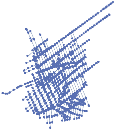
With all the roads data at hand, let’s consider a giant graph formed by all these nodes and ways . The nodes are vertices; the ways between two consecutive nodes are edges . Later on, we will take a portion of this giant graph that topologically equivalent to the graph generated from our character. To form such a giant graph, apply UndirectedEdge function onto every pair of two consecutive nodes. In other words, connect every pair of two consecutive nodes by edges .
For each pair of the two consecutive nodes, connect them to form the giant graph.
In[]:=
waysEdges=Flatten[UndirectedEdge@@@Partition[#,2,1]&/@Values[nodesAtCrossings]];vertexcoord=#[[1]]&/@VertexList[Graph@waysEdges];roadsGraphVertexCoords=Graph[waysEdges,VertexCoordinatesvertexcoord];
See how giant the entire road graph is? About three thousand vertices! Let’s play a trick to make the graph a little organized.
Graph[roadsGraphVertexCoords]//VertexCount
Out[]=
3246
The trick is to add each edge a weight, where weights are proportional to the real road distances. In this way, when showing the graph with specified option “EdgeWeight -> weights”, the graph will prioritize showing more weighted edges. Later on, when we place our character onto this giant graph, you will find why the trick works.
Compute the weights by applying GeoDistance function to edges. Note that we do not care about the quantity unit, only the magnitude: weights are relative measurements here.
In[]:=
weights=QuantityMagnitude[GeoDistance@@@(EdgeList[roadsGraphVertexCoords]),"Meters"];
Visualize the giant map graph:
roadsGrahpVertexCoordsWeighted=Graph[roadsGraphVertexCoords,EdgeWeightweights]
Out[]=
Fantastic! Look how grid-like downtown Manhattan is turned into a weighted graph.
Next, store the processed geographical data into an association. The values of the association are the different parts of the dataset such as the map graph or highway nodes . Later on, we may want to fetch, for example, the highway nodes by the key "HighwayNodes" .
Construct the mapData association:
In[]:=
mapData=<|"Origin"origin,"Radius"radius,"HighwayNodes"highwayNodes,"HwgWeighted"roadsGrahpVertexCoordsWeighted,"NodesAtCrossings"nodesAtCrossings|>;
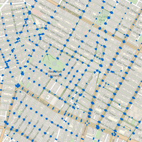
Visualize the nodes and ways in the region within 1 mile centered at New York University.
GeoGraphics,Line/@mapData[["NodesAtCrossings"]],,Point[mapData[["HighwayNodes"]]],GeoRangeGeoDisk[origin,radius]
Out[]=
Okay, pause the geo-processing a bit -- let’s move on to process our desired character.
Section 2 Turn a Character into a Thinned Region
Section 2 Turn a Character into a Thinned Region
Given a character in String type, we first turn the character into a 2D picture; then we reduce to 1D lines.
In[]:=
rasterSize=625;
In[]:=
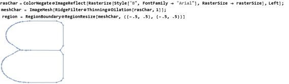
rasChar=ColorNegate@ImageReflect[Rasterize[Style[character,FontFamily"Arial"],RasterSizerasterSize],Left];meshChar=ImageMesh[RidgeFilter@Thinning@rasChar];region=RegionBoundary@RegionResize[meshChar,{{-.5,.5},{-.5,.5}}];Grid;
Visualize the key steps turning a character into the boundary of a region:
Out[]=

So far, we’ve successfully turned a 2D region into 1D lines.
Section 3 Turn the Region into a Geo-referenced Graph
Section 3 Turn the Region into a Geo-referenced Graph
From the previous section, the character string is converted to the boundary of a region. Note that the boundary is consisted of lines and points. In other words, the “MeshPrimitives” of the boundary in 1D is just lines. Taking the advantages of the boundary, we convert the region into a graph.
Apply geo-referenced transformation to the region
Apply geo-referenced transformation to the region
In order for an arbitrary region to geographically match our region of interest, we apply the three transformation on to the character region: translation, scale, and rotation.
Translate the region to the latitude and longitude of the desired location:
In[]:=
translated=Translate[region,origin["LatitudeLongitude"]];
Scale the region based on projection distortion from GeoGridUnitDistance:
According to Open Street Map
According to Open Street Map
In[]:=
scaled=RegionResize[translated,2radius/GeoGridUnitDistance["Equirectangular",origin,"N"]];
Rotate the region by the rotationAngle given:
In[]:=
rotated=Rotate[scaled,rotationAngle];
After transformation, extract the lines from the our region boundary:
In[]:=
lines=MeshPrimitives[rotated,1];
Connect the lines by UndirectedEdge:
lineGraph=Graph[Apply[UndirectedEdge,Sequence@@#]&/@lines]
Out[]=
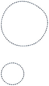
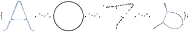
Observe that the lineGraph has multiple components because our region “A” has two closed region: the outline and the triangle inside. We only need the outline for drawing a morphology on street map. How do we know which is the outline one? According to the ConnectedGraphComponents function documentation, the largest component is placed first. The outline is the longest, so the largest.
Therefore, extract the first element from the lineGraph:
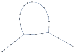
meshgraph=ConnectedGraphComponents[lineGraph][[1]]
Out[]=
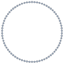
Watch that the meshgraph of the region “A” is a full circle. Why? Because the outline of the character “A” is exactly a topological ring! In fact, the meshgraph of all of the 26 English alphabet character regions are just a ring -- they are topological equivalent because regions are outlines!
So far all the components in the meshgraph are evenly distributed. Group the meshgraph in to clusters, and merge closed nodes into one nodes. This node is a representative for a neighbor cluster.
Define a magical value nearbyThreshold. Multiple nodes within the nearbyThreshold value are considered as “neighbors”. Each cluster forms a graph.
nearbyThreshold=2radius*0.015/GeoGridUnitDistance["Equirectangular",mapData[["HighwayNodes"]][[1]],"NE"];nearestGraph=NearestNeighborGraph[VertexList[meshgraph],{All,nearbyThreshold}]
Out[]=
For each cluster in the neighbor graph, merge the neighbor vertices into single vertex:
meshgraph=VertexReplace[meshgraph,Flatten[Map[connectedVertices(#connectedVertices[[1]]&/@connectedVertices),ConnectedComponents[nearestGraph]]]]
Out[]=
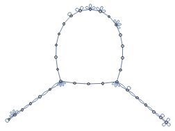
See how the previous outline transforms into a morphologically satisfying graph:
In[]:=
See the last graph has lots of self-looping nodes? These are the heritage from neighbor-merging. Don’t worry, we will fix it in next section.
Section 4 Bind the Character Graph to the Map Graph
Section 4 Bind the Character Graph to the Map Graph
Now we have our character graph and map graph ready. A character graph stores the character morphology, while a map graph stores the geographical information. Okay, ready to bind the character graph and map graph together -- a third graph, like a child of the previous two, carries all the good properties. With the blended properties at one graph, it will be sufficient to draw the character on the map.
According to the RegionNearest function documentation, it “gives a point in the region that is nearest the point”. In our case, the region is all the Point objects derived from highway nodes. These Point Objects, a.k.a. the region, acting like a magnet, pull over the nearest arbitrary vertices on the character graph. Once a vertex is picked up as the “nearest”point to the Point object, they are bonded. For each binding pair points, the vertex will be replaced by the Point object. Remember our Point objects stores geographical info, while our vertex does not. Hence the vertex replacement “steals” the geographical info through the bond, while still keeping morphological connections. In this way, we bind the character graph to the map graph.
Let’s step through the code to see the beautiful binding.
Region “magnet”:
In[]:=
Point[Values@mapData[["HighwayNodes"]][[All,1]]];
In[]:=
regionNearestNodes=RegionNearest[Point[Values@mapData[["HighwayNodes"]][[All,1]]]];
Set the rule to apply the RegionNearest function:
In[]:=
(#->regionNearestNodes[#])&;
Map the function onto vertices. Here’s the binding happening:
In[]:=
(#->regionNearestNodes[#])&/@VertexList[meshgraph];
Replace the vertices into geo-referenced points :
replaced=VertexReplace[meshgraph,(#->regionNearestNodes[#])&/@VertexList[meshgraph]]
Out[]=
Note that there are quite a lot of self-looping edges at some vertices. Self-looping edges do not help to construct a shortest tour later on, so we delete these edges using EdgeDelete and DeleteDuplicatesBy[Sort]] functions.
Delete the self-looping edges, wrap each vertex up to GeoPosition object:
In[]:=
trimGraph=EdgeDelete[replaced,x_x_];nng=Graph[EdgeList[trimGraph]//DeleteDuplicatesBy[Sort]];
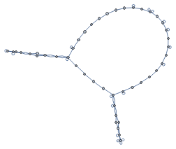
For now, each vertices is barely a pair of numeric coordinates. Wrap each of them up to GeoPosition object using VertexReplace function.
Delete the self-looping edges, wrap each vertex up to GeoPosition object, and display the result:
nng=VertexReplace[nng,(#->GeoPosition[#])&/@VertexList[nng]]
Out[]=
The graph looks cleaner. It' s fairly usable to construct a tour. Let' s move on.
Section 5 Assign a Shortest Tour
Section 5 Assign a Shortest Tour
So far we have generated a clean, morphological, geo-referenced graph. Considering the real road segments distances, we would like to minimize the total distance while still traversing through every vertices. A well-built algorithm for solving the Chinese Postman Problem assists us to generate an ordered list of edges. Threading the edges gives a graph that will 1) visit all the edges at least once; 2) minimize the total distance.
Note that the list of edges we generated from above may contain repeated edge because, think about you handwrite certain kinds of character in ONE line: drawing it without repeating parts may be impossible, such as characters “T” and “Y”.
Note that the list of edges we generated from above may contain repeated edge because, think about you handwrite certain kinds of character in ONE line: drawing it without repeating parts may be impossible, such as characters “T” and “Y”.
Use the FindPostmanTour function to generate an ordered lists of edges:
In[]:=
postmanTour=FindPostmanTour[nng][[1]];
Generate a sequence of vertices to visit by appending the second vertex of the previous edge to the first vertex:
In[]:=
postmanTourNodes=Append[postmanTour[[All,1]],postmanTour[[-1,2]]];
The list of nodes above may contain repeated nodes for the same reason.
Within two consecutive nodes on the street map, usually there are more than one connection way. Therefore, for each two consecutive nodes #1, #2 in postmantTourNodes, find the shortest path from source #1 to target vertex #2 in the weighted highway graph. We retrieve the weighted graph through mapData[[“HwgWeighted”]].
Within two consecutive nodes on the street map, usually there are more than one connection way. Therefore, for each two consecutive nodes #1, #2 in postmantTourNodes, find the shortest path from source #1 to target vertex #2 in the weighted highway graph. We retrieve the weighted graph through mapData[[“HwgWeighted”]].
Construct a shortest path between two consecutive nodes using FindShortestPath function:
In[]:=
shortestPath=FindShortestPath[mapData[["HwgWeighted"]],#1,#2]&@@@postmanTour;
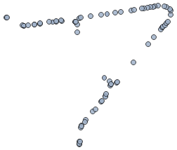
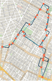
The shortest tour traces through a character “A” around New York University. We’re all set, let’s draw! Whoo hoo!
Visualize the shortest path, the vertices we visit, and the character graph on one map:
GeoGraphicsThickness[.01],,Line[#]&/@shortestPath,Thickness[.006],,Line[postmanTourNodes],,PointSize[Large],Point/@postmanTourNodes
Out[]=
Section 6 Integrate Sections into Functions for Reusability
Section 6 Integrate Sections into Functions for Reusability
Now we succeed in drawing one tour graph specific to an origin, a radius, a character and the rotation angle. What if we want to compare the multiple results, say, at different angles? At different origin, or try with different characters? That will be a disaster if you manually change the variables defined in section 1. Here we introduce a programming strategy -- encapsulation -- to mange our sections of codes in a more structured way.
What we going to do next, is to integrate the previous sections, or parts of a section into functions. Later on, we may easily call functions by passing the arguments of interested, paving the way for further code testing and robust program.
What we going to do next, is to integrate the previous sections, or parts of a section into functions. Later on, we may easily call functions by passing the arguments of interested, paving the way for further code testing and robust program.
Define a function that requests the geographical data within region of interest
Define a function that requests the geographical data within region of interest
Define series of functions that extract the nodes and ways
Define series of functions that extract the nodes and ways
Define a function that turns a Character into a Thinned Region
Define a function that turns a Character into a Thinned Region
Define a function that turns the Region into a Geo-referenced Graph
Define a function that turns the Region into a Geo-referenced Graph
Define a function that binds the Character Graph to the Map Graph
Define a function that binds the Character Graph to the Map Graph
Define a function that assigns a Shortest Tour
Define a function that assigns a Shortest Tour
Define a function that visualize all the nodes and ways within our region of interest:
Define a function that visualize all the nodes and ways within our region of interest:
All functions at one call: draw
All functions at one call: draw
Wrap up all the procedures above into one single function. Then we can simply call draw function once and get the tour!
In[]:=
draw[mapData_Association,char_String,rot_Quantity]:=Module[{charGraph,geoCharGraph,nearestNodesGeoGraph,postmanTour,postmanTourNodes,shortestPath},charGraph=characterGraph[char];geoCharGraph=geoCharacterGraph[charGraph,mapData[["Origin"]],mapData[["Radius"]],rot,mapData[["HighwayNodes"]]];nearestNodesGeoGraph=nearestNodesGraph[geoCharGraph,mapData[["HighwayNodes"]]];nearestNodesGeoGraph=VertexReplace[nearestNodesGeoGraph,(#->GeoPosition[#])&/@VertexList[nearestNodesGeoGraph]];postmanTour=FindPostmanTour[nearestNodesGeoGraph][[1]];postmanTourNodes=Append[postmanTour[[All,1]],postmanTour[[-1,2]]];shortestPath=shortestPathTour[postmanTour,mapData[["HwgWeighted"]]];visualizeEverything[shortestPath,postmanTourNodes]]
Function overloading: allows draw function takes in another argument list.
In[]:=
draw[ori_GeoPosition,rad_Quantity,char_String,rot_Quantity]:=draw[getMapData[ori,rad],char,rot]
Section 7 Fun examples
Section 7 Fun examples
Recall that we defined four key variables in the previous example. We can actually play around with these variables and see different outputs :-)
Creative mind! Here can be really fun!
Creative mind! Here can be really fun!
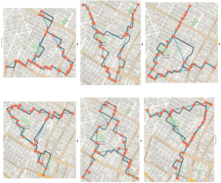
Example by rotation angle
Example by rotation angle
Rotate the angle by 60 degrees for 6 times, leaving the other three variables unchanged:
draw[origin,radius,"A",Quantity[#,"AngularDegrees"]]&/@Range[30,330,60]
Out[]=
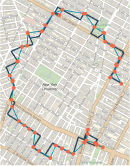
Example by character
Example by character
Draw a character C at counterclockwise 60 degree rotation angle:
draw[origin,radius,"C",Quantity[-60,"AngularDegrees"]]
Out[]=
Example by location
Example by location
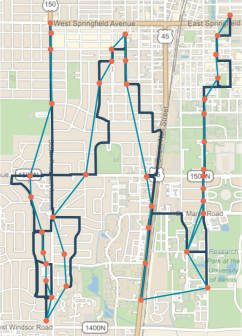
Draw a character “W” centered at Wolfram office at Illinois:
In[]:=
il=GeoPosition[{40.098903,-88.249638}];
draw[il,Quantity[1,"Miles"],"W",Quantity[-90,"AngularDegrees"]]
Out[]=
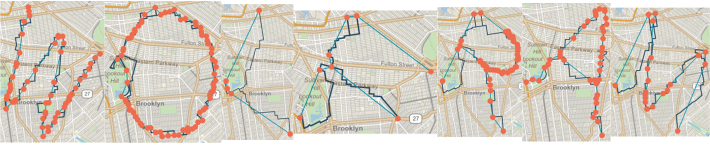
HAPPY
HAPPY
In[]:=
draw[origin,Quantity[2,"Miles"],#,Quantity[-60,"AngularDegrees"]]&/@Characters["HAPPY"]
Out[]=
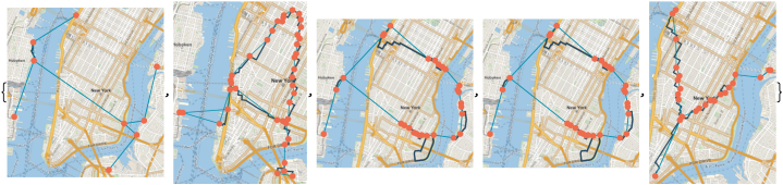
WOLFRAM
WOLFRAM
md=getMapData[GeoPosition@Entity["City",{"NewYork","NewYork","UnitedStates"}],Quantity[2,"Miles"]];imgs=draw[md,#,Quantity[-60,"AngularDegrees"]]&/@Characters["WOLFRAM"];Row[Show[#,ImageSize->Small]&/@imgs]
Out[]=
Section 8 Limitations and Future Works
Section 8 Limitations and Future Works
1
.Now the entire methodology is integrated into one single function draw. Future developers may iteratively call draw function over various argument list. Continued from the rotate-by-60 example in the section 7, developers may define a measurement for the performance at each iteration. For example, compute the total number of turns each iterations. Define a threshold, say 10 turns. Those that have total number of turns under 10 turns are considered good practices. There are many designs to play around with the iterations and measurements of the function call. We encourage the readers and users download this notebook, modify arguments in draw, and apply draw functions in various strategies.
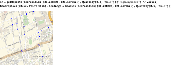
2
.For different city inside or outside of the United States, the overpass API may return a dataset that contains limited amount of usable highway nodes, and thus potentially lower the possibility to find a desired tour.
◼
For example, at the central area of Shanghai, China, the dataset returns sparse nodes; at some crossroads, there is no nodes.
◼
3
.Turning a character into a region does not work for every English alphabet letter (section 2). For example, character “B” results an error from RegionResize function:
rasChar=ColorNegate[ImageReflect[Rasterize[Style["B",FontFamily"Arial"],RasterSizerasterSize],Left]];meshChar=ImageMesh[RidgeFilter[Thinning[rasChar]]];region=RegionBoundary[RegionResize[meshChar,{{-0.5,0.5},{-0.5,0.5}}]];RegionResize::invRegionBoundary::reg
RegionResize: The argument { ... } in RegionResize is not a correctly specified region
This is because, the ImageMesh function fails to turn the 2D region into 1D line. The error message gives “The boundary curves self-intersect or cross each other...”. Perhaps the Thinning function turns some parts of the region so thin that the boundary of the region self-interact.
BoundaryMeshRegion : The boundary curves self - intersect or cross each other in ...
One proposed solution to the over-thinned region is to apply a Dilation to it, making it “fatter”:
◼
4
.Mentioning in the section 3, all the 26 English alphabets can generate closed-ring boundaries. That is because the alphabets are morphologically independent. Unlike characters in other languages, especially in Asian languages, characters may contain separate parts. For example, my last name “陈” (character code: 38472) is a glyph consisted of four separated components. If we follow the methodologies in this project, the function ConnectedComponents[lineGraph][[1]] will get rid of the rest components. Future developers may consider generalize the methodology to glyph that consisted of multiple separate components.
FromCharacterCode[38472]
Out[]=
陈
Keywords
Keywords
◼
Image Processing
◼
Geographic processing
◼
Street Map
◼
Graph Theory
◼
Network
◼
Topology
◼
Chinese Postman Tour
◼
Shortest Path
◼
Open Street Map
◼
Character
Acknowledgment
Acknowledgment
Special thanks to Dr. Stephen Wolfram. He defined my project at an instance, pointed me out the core challenge during the progress and highly encouraged me to keep on going with the project. His words are impressively inspiring. It’s my honor to have him consulted.
Sincerely appreciate Jesse Galef, my dear Mentor, who gave me a hand when we started everything from scratch. He helped me construct the foundation of this project: map graph and character graph. During our meetings, he demonstrated nice examples. When I was anxious, he was always calm, patiently experiments with blocks of code. I was reassured by his actions.
A thousand thanks to dear Jesse Friedman, TA at our school. His blog post “Taking the Cerne Abbas Walk: From Conceptual Art to Computational Art” inspired me. I borrowed some brilliant ideas for constructing functions and general methodologies. During the school, Jesse was at all time patient at answering all my questions in nice details. His decent suggestions are utterly useful. He is talented, humble and polite, and his personalities inspire me quite much. At so many moments I was disappointed at myself in front of challenges, he kept guiding me to look at positive sides. I remember, at one start of our meeting, I fixed my earphone track. His humor lit up the room: “In the first thirty seconds we’ve already fixed one problem. It was an efficient meeting :-) “ I deeply enjoyed every conversation with Jesse.
Thanks to Christopher Wolfram, who introduced me to Open Street Map data resource, which is essentially the starting point of this project.
Our coordinators Erin Cherry and Mads Bahrami stood for the longest -- they took up the whole program since the recruiting. During the interview with Mads, he double-checked making sure I cleared out all the questions, which brought me kindness from other end of the virtual world. Erin and Mads managed our logistics, cleared up all the questions, gave kind reminders at important dates. They deserve a fine rest! (So as others!)
Our nice TA Siliva Hao solved my network problem, answered lots of questions perfectly, proofread at my final version of project. She gave important suggestions to me. Thank you, Silvia!
Thank you for all the TAs, mentors, lecturers and students! Without any of you we can’t make it through today.
July 14, 2 AM EST,
Shanghai
References
References
Chinese Postman Tour Problem
Chinese Postman Tour Problem
◼
Weisstein, Eric W. “Traveling Salesman Problem.” From MathWorld--A Wolfram Web Resource. https://mathworld.wolfram.com/TravelingSalesmanProblem.html
◼
Wolfram Research (2012), FindPostmanTour, Wolfram Language function, https://reference.wolfram.com/language/ref/FindPostmanTour.html (updated 2015).
Find Shortest Path
Find Shortest Path
◼
Wolfram Research (2010), FindShortestPath, Wolfram Language function,https://reference.wolfram.com/language/ref/FindShortestPath.html (updated 2015).
General
General
◼
Friedman, Jesse (2019), Taking the Cerne Abbas Walk: From Conceptual Art to Computational Art, Wolfram Language function, https://blog.wolfram.com/2019/08/08/taking-the-cerne-abbas-walk-from-conceptual-art-to-computational-art/