Boids is a simple model of flocking behavior which has been used to simulate the movements of birds in a flock, fish in a school, etc. Boids is one of the classic examples of emergent behavior, with simple and local rules producing complex global behavior.

Back in 2014 (when I was 15), I wrote a C program for efficiently simulating boids in an arbitrary number of dimensions. My original goal was to experiment with OpenGL through GLFW, but I ended up using the code more for analysis than for visualization. Above is a screencapture of the C program with three species which try to avoid each other:

Having multiple “species” is nice because it keeps them from all forming into one big static flock, and because it produces nice fission-fusion behavior.

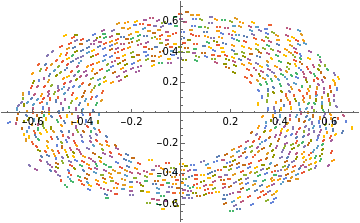
It gets more interesting as you vary the parameters which determine the behavior of the boids. For example, this figure shows a frame from a simulation where each boid has a random visibility radius, as indicated by the color of the dot:

The blue boids have a lower visibility range, while the red ones have a higher visibility range. You can see how the boids with low visibility range end up in the center, while those with a high visibility range end up on the exterior, presumably because they can see the predators in the center and choose to avoid it. More generally, the goal was to see how the global behavior of the flock is affected by changes to the parameters of individual agents. I don’t have concrete enough results to warrant a proper writeup, but here is one of my working notebooks which shows some initial findings.

Init

Needs["CCompilerDriver`"]

SetDirectory[NotebookDirectory[]];

libraryPath=CreateLibrary[{"cfiles/link.c","cfiles/boids.c"},"boids","IncludeDirectories"{Directory[]<>"/cfiles"}];Print[libraryPath]

/Users/christopher/Library/Mathematica/SystemFiles/LibraryResources/MacOSX-x86-64/boids.dylib

runBoids=LibraryFunctionLoad[libraryPath,"runBoids",{Integer(*stepcount*),Integer(*stepstoreturncount*),{Real,2}(*initialpositions*),{Real,2}(*initialvelocities*),{Real,2}(*parameters*)},{Real,3}]

LibraryFunction

Function name: runBoids

Argument count: 5



Without Predators

initPos=RandomReal[{-1,1},{100,1}];initVel=RandomReal[{-1,1},{100,1}];parameters=Table[{10(*alignment*),1(*seperation*),1(*cohesion*),0(*species*),1(*mass*),0.3(*visibilityradius*),0.01(*maxvelocity*),0.001(*maxacceleration*),0.025(*seperationradius*),1.0(*fear*),0(*predatorframes*),10(*framestodeath*)},{100}];

initPos=RandomReal[{-1,1},{1000,2}];initVel=RandomReal[{-1,1},{1000,2}];parameters=Table[{10(*alignment*),1(*seperation*),1(*cohesion*),0(*species*),1(*mass*),0.3(*visibilityradius*),0.01(*maxvelocity*),0.001(*maxacceleration*),0.025(*seperationradius*),1.0(*fear*),0(*predatorframes*),10(*framestodeath*)},{1000}];

initPos=RandomReal[{-1,1},{1000,2}];initVel=RandomReal[{-1,1},{1000,2}];parameters=Table[{10(*alignment*),1(*seperation*),10(*cohesion*),0(*species*),1(*mass*),0.3(*visibilityradius*),0.01(*maxvelocity*),0.001(*maxacceleration*),0.025(*seperationradius*),1.0(*fear*),0(*predatorframes*),10(*framestodeath*)},{1000}];

steps=runBoids[1000,1000,initPos,initVel,parameters];

AbsoluteTiming[runBoids[1000,2,initPos,initVel,parameters];]

{0.089834,Null}

0.079085`*(100^3)/60/60/4

5.49201

7.34016`

10^3*10/60/60//N

2.77778

10.706806`

center=Mean[Catenate[steps]];distances=EuclideanDistance[center,#]&/@Catenate[steps];

Histogram[distances]

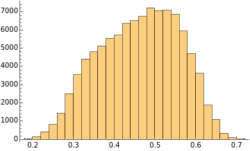
Mean[distances]

0.461488

StandardDeviation[distances]

0.097804

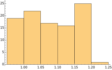
Histogram[Norm/@(Subtract@@Reverse@steps[[-2;;]])]

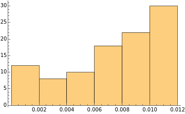
A reasonable measure of something:

Mean[Norm/@(Subtract@@@steps[[All,-2;;]])]

0.00566809

Histogram[Norm/@(Subtract@@@steps[[All,-2;;]])]

ListPlot@steps[[All,-2;;]]

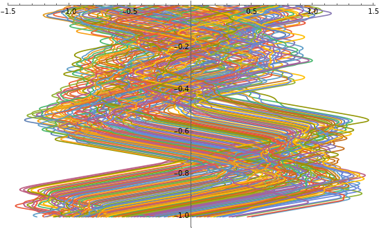
ListLinePlot[MapIndexed[{#1,-First[#2]/1000}&,#]&/@steps[[All,All,1]],PlotRange{Automatic,All}]

Phase Diagram

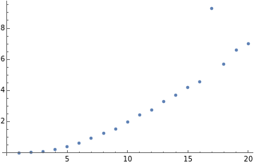
times=Table[Module[{initPos,initVel,parameters},initPos=RandomReal[{-1,1},{n,2}];initVel=RandomReal[{-1,1},{n,2}];parameters=Table[{10(*alignment*),1(*seperation*),1(*cohesion*),0(*species*),1(*mass*),0.3(*visibilityradius*),0.01(*maxvelocity*),0.001(*maxacceleration*),0.025(*seperationradius*),1.0(*fear*),0(*predatorframes*),10(*framestodeath*)},{n}];AbsoluteTiming[runBoids[1000,2,initPos,initVel,parameters]][[1]]],{n,1,1000,50}]

{0.000273,0.022402,0.086847,0.212882,0.388209,0.649892,0.946567,1.27527,1.54806,2.00375,2.4247,2.74454,3.28513,3.69716,4.22439,4.57997,9.25714,5.70732,6.61105,7.00996}

ListPlot[times]

if=Interpolation[Transpose[{Range[1,1000,50],times}]]

InterpolatingFunction

Domain: {{1.,951.}}

Output: scalar



100^3*if[200]/3/60/60

36.6844

Dimensions[steps2]

{200,1000,2}

Transpose[steps2][[-500;;]]

{{{-1.05837,-0.789296},{-0.24979,-0.0763523},{2.79794,-0.251807},{1.59536,0.474895},{-0.668717,0.474544},{3.319,-0.526554},{-0.817533,-0.88365},{-0.0897784,0.336451},

⋯184⋯

,{1.59199,0.0797473},{3.33536,-0.48146},{-0.565913,0.0760649},{-1.1367,-0.881877},{3.29441,-0.380596},{-0.932509,-0.784458},{3.28443,-0.501919},{1.31412,0.396489}},

⋯498⋯

⋯1⋯

}}

large output

show less

show all

set size limit...

{Mean[#],Median[#],StandardDeviation[#]}&/@Map[Norm,Subtract@@@Partition[Transpose[steps2][[-500;;]],2,1],{2}]

ListPlot[Mean/@Map[Norm,Subtract@@@Partition[Transpose[steps2][[-500;;]],2,1],{2}]]

Dimensions[Subtract@@@Partition[Transpose[steps2][[-500;;]],2,1]]

{499,200,2}

Dimensions[steps2[[All,-500;;]]]

{200,500,2}

Space3:

LaunchKernels[6]

{KernelObject[1,local],KernelObject[2,local],KernelObject[3,local],KernelObject[4,local],KernelObject[5,local],KernelObject[6,local]}

Now+

16.3764245`

min

Thu 21 Sep 2017 11:28:20GMT-7.

space3=ParallelTable[Module[{initPos,initVel,parameters,steps,norms,n,s},s=1;n=200;initPos=RandomReal[{-1,1},{n,2}];initVel=RandomReal[{-1,1},{n,2}];parameters=Table[{a(*alignment*),s(*seperation*),c(*cohesion*),0(*species*),1(*mass*),0.3(*visibilityradius*),0.01(*maxvelocity*),0.001(*maxacceleration*),0.025(*seperationradius*),1.0(*fear*),0(*predatorframes*),10(*framestodeath*)},{n}];steps=runBoids[1000,500,initPos,initVel,parameters];norms=Map[Norm,Subtract@@@Partition[Transpose[steps],2,1],{2}];{Mean[#],Median[#],StandardDeviation[#]}&/@norms],{c,0,10,10/100},{a,1,21,20/100}];

Now

Thu 21 Sep 2017 11:32:18GMT-7.

Space4:

space4=ParallelTable[Module[{initPos,initVel,parameters,steps,norms,n,s},s=1;n=200;initPos=RandomReal[{-1,1},{n,2}];initVel=RandomReal[{-1,1},{n,2}];parameters=Table[{a(*alignment*),s(*seperation*),c(*cohesion*),0(*species*),1(*mass*),0.3(*visibilityradius*),0.01(*maxvelocity*),0.001(*maxacceleration*),0.025(*seperationradius*),1.0(*fear*),0(*predatorframes*),10(*framestodeath*)},{n}];steps=runBoids[1000,500,initPos,initVel,parameters];norms=Map[Norm,Subtract@@@Partition[Transpose[steps],2,1],{2}];{Mean[#],Median[#],StandardDeviation[#]}&/@norms],{c,0,10,10/100},{a,1,21,20/100},100];

Space:

Table[Module[{initPos,initVel,parameters,steps,norms,n},n=200;initPos=RandomReal[{-1,1},{n,2}];initVel=RandomReal[{-1,1},{n,2}];parameters=Table[{a(*alignment*),s(*seperation*),c(*cohesion*),0(*species*),1(*mass*),0.3(*visibilityradius*),0.01(*maxvelocity*),0.001(*maxacceleration*),0.025(*seperationradius*),1.0(*fear*),0(*predatorframes*),10(*framestodeath*)},{n}];steps=runBoids[1000,2,initPos,initVel,parameters];norms=Norm/@(Subtract@@@steps[[All,-2;;]]);{Mean[norms],Median[norms],StandardDeviation[norms]}],{c,0,10,10/100},{a,1,21,20/100},{s,1,11,10/100}]$Aborted

Space2:

$Aborted

Will finish at 5:30am on Tuesday the 19th

Norm/@(Subtract@@@steps[[All,-2;;]])

{0.01,0.01,0.01,0.00987525,0.01,0.01,0.01,0.01,0.01,0.01,0.01,0.01,0.01,0.01,0.01,0.01,0.01,0.01,0.01,0.01,0.01,0.01,0.01,0.01,0.01,0.01,0.01,0.00865782,0.01,0.01,0.01,0.01,0.01,0.01,0.01,0.01,0.01,0.00911974,0.01,0.01,0.01,0.01,0.01,0.01,0.01,0.01,0.01,0.01,0.01,0.01,0.01,0.01,0.01,0.01,0.01,0.01,0.01,0.01,0.01,0.01,0.01,0.01,0.01,0.01,0.01,0.01,0.01,0.01,0.01,0.01,0.01,0.01,0.01,0.01,0.01,0.01,0.01,0.01,0.01,0.01,0.01,0.01,0.01,0.01,0.01,0.01,0.00705106,0.01,0.01,0.01,0.01,0.01,0.01,0.01,0.01,0.01,0.01,0.01,0.01,0.01}

space=Get[FileNameJoin[{NotebookDirectory[],"space.wl"}]];

space2=Get[FileNameJoin[{NotebookDirectory[],"space2.wl"}]];

space3=Get[FileNameJoin[{NotebookDirectory[],"space3.wl"}]];

Get[FileNameJoin[{NotebookDirectory[],"space4.mx"}]];

Dimensions[space]

{101,101,101,3}

Dimensions[space3]

{101,101,499,3}

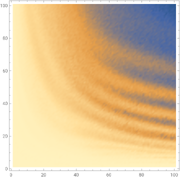
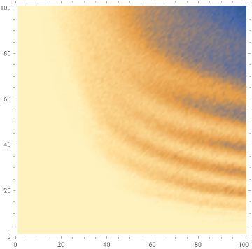
means=Map[Mean,space4[[All,All,All,All,1]],{2,3}];

ImageAdjust@Image@means

ListPlot3D[means]

ListAnimate[Table[ImageAdjust@Image[Map[Mean,space4[[All,All,n,All,1]],{2}],ImageSize400],{n,1,100,1}],AnimationRunningFalse]

Out[]=

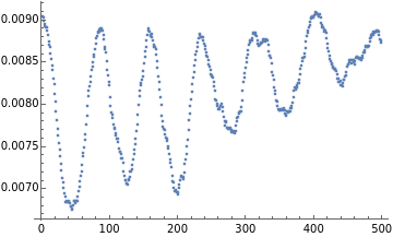
ListPlot@space3[[100,52,All,1]]

ListAnimate[Table[ImageAdjust@Image[space3[[All,All,n,1]],ImageSize400],{n,1,499,1}],AnimationRunningFalse]

Out[]=

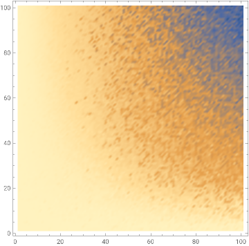
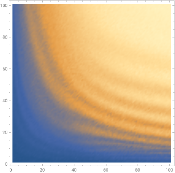
ListDensityPlot@Map[Total,space3[[All,All,All,1]],{2}]

ListPlot3D[Map[Total,space3[[All,All,All,1]],{2}]]

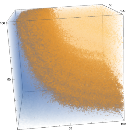
ListDensityPlot3D@space[[All,All,All,1]]

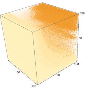
ListDensityPlot3D@space[[All,All,All,3]]

ListPlot3D[Map[Total,space[[All,All,All,1]],{2}]]

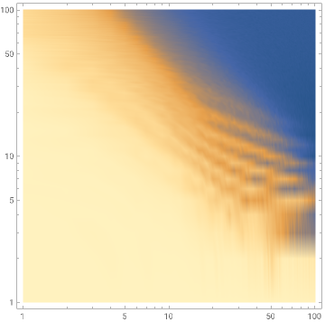
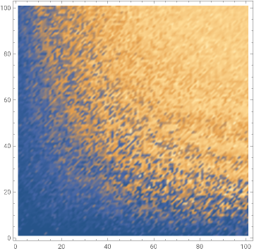
ListDensityPlot[Map[Total,space2[[All,All,All,1]],{2}],ScalingFunctions{"Log","Log"}]

ListDensityPlot[Map[Total,space2[[All,All,All,1]],{2}]]

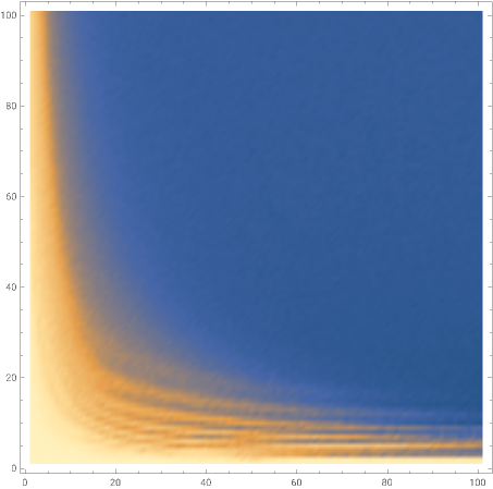
ListDensityPlot[Map[Total,space[[All,All,All,1]],{2}]]

ListDensityPlot[Map[Total,space[[All,All,All,2]],{2}]]

ListDensityPlot[Map[Total,space[[All,All,All,3]],{2}]]

ListDensityPlot@space[[All,All,50,3]]

With Predators

Variable visibility radii:

initPos=RandomReal[{-1,1},{1000,2}];initVel=RandomReal[{-1,1},{1000,2}];parameters=Table[{10(*alignment*),1(*seperation*),1(*cohesion*),RandomChoice[{0,1,3,4}](*species*),1(*mass*),RandomReal[{0.2,0.5}](*visibilityradius*),0.01(*maxvelocity*),0.001(*maxacceleration*),0.025(*seperationradius*),1.0(*fear*),0(*predatorframes*),10(*framestodeath*)},{1000}];

steps=runBoids[10000,10000,initPos,initVel,parameters];

boidColors=ColorData["TemperatureMap"]/@Rescale[parameters[[All,6]]];

Manipulate[Graphics[MapThread[{#2,Point[#1]}&,{steps[[All,n]],boidColors}],PlotRange2],{n,1,Length@First@steps,1}]

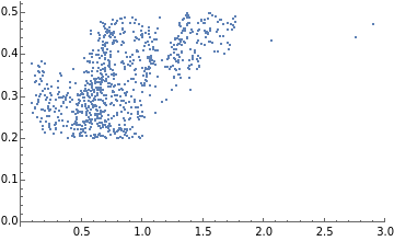
center=Mean[steps[[All,-1]]];ListPlot[Transpose[{EuclideanDistance[center,#]&/@steps[[All,-1]],parameters[[All,6]]}],PlotRange{{0,3},All}]

Manipulate[center=Mean[steps[[All,n]]];ListPlot[Transpose[{EuclideanDistance[center,#]&/@steps[[All,n]],parameters[[All,6]]}],PlotRange{{0,3},All}],{n,1,Length@First@steps,1}]

Graphics[MapThread[{#2,Point[#1]}&,{steps[[All,10000]],boidColors}],PlotRange2]

CITE THIS NOTEBOOK

Phase diagram of boids: complex global behavior emerging from simple local rules
by Christopher Wolfram
Wolfram Community, STAFF PICKS, April 30, 2024
https://community.wolfram.com/groups/-/m/t/3166791