Abstract

We report work-in-progress with conservative, geometric, discrete, variational integrators on Lie groups — modern techniques for simulation and control software. The current notebook successfully applies geometric integration to a benchmarking example — A non-isotropic top that spontaneously exhibits the intermediate-axis phenomenon pursuant to the tennis-racket theorem.[8] The geometric integrator CGDVIE3 (conservative, geometric, discrete, variational integrator on SE(3)) conserves energy for this benchmark at least as well as Runge-Kutta-4 (RK4) over quaternions, but with a time step 3 times larger.

The long-term objective of this series of notebooks is to integrate the 4-degree-of-freedom inverted spherical pendulum (4DISP) with CGDVIE3. 4DISP is surprisingly difficult given that the 2-DOF inverted circular pendulum (2DICP) is an undergraduate exercise. Numerically, 2DICP is easily solved using any of the methods below that failed on 4DISP.[15] The final objective — 4DISP on CGDVIE3 — awaits further research outlined below. In this notebook, we exhibit intermediate results:

◼

RK4 on quaternions fails spectacularly 4DISP, even with painfully small, sub-millisecond time steps. The integrator is conclusively shown at fault; the dynamical model is correct.

◼

Rewriting 4DISP in pitch-cone-roll coordinates avoids singularity at the North pole, as with quaternions. We apply Mathematica’s NDSolve to the standard Euler-Lagrange equations. This works well, but does not export out of Mathematica. For our purposes, it furnishes ground truth for later developments.

◼

Next stop is a simple discrete Lagrangian integrator on pitch-cone-roll coordinates — Discrete Euler-Lagrange Equations (DELE).[10] This works plausibly but disappoints. Like RK4, it requires fine time steps, making it too slow.

◼

Next stop is CGDVIE3. Coding it requires a deep swim in manifold theory, topic of other notebooks of mine. We get it working on the non-isotropic top. It is most promising for 4DISP, but we must formulate an adjoint representation for force in the cotangent bundle, and that work is not done yet.

Prior Failures


The Future: Discretized Lagrangians on Lie Groups

Contemporary integrators embody the following features:

◼

The Lagrangian is discretized before applying the variational principle, resulting in discrete, reduced Euler-Poisson equations (DREPEs). Contrast discretized Euler-Lagrange equations, wherein the variational principle is applied before discretizing. Discretizing first is the contemporary approach, supported by many dissertations and papers from the shop of the late Jerrold E. Marsden and his students at Caltech (citations inline). A similar approach pertains to Hamiltonian formulations.

◼

The intrinsic configuration manifold of a rigid body is SE(3). Typical textbooks present rigid-body mechanics in Euler angles or quaternions. Euler angles inhabit the surface of a 3-toroid and rotation quaternions inhabit the interior of a 3-ball or the surface of the unit 4-sphere. Neither manifold has a similar structure to SE(3). Integrating Euler angles invites gimbal lock. Integrating either Euler angles or quaternions invites non-conservation. Integrating DREPEs on the correct manifold automatically — in theory — conserves energy, momentum, and angular momentum pursuant to the discrete Noether’s theorem.[9][10] We find difficulties in the concrete implementations below.

The theoretical arguments in favor of integrating DREPEs on the appropriate manifold are compelling. Integrators that do so are called “discrete variational integrators on Lie groups” or “geometric discrete variational integrators.” The particular integrator we need is CGDVIE3 — conservative, geometric, discrete, variational integrator on SE(3).

Quaternions and RK4

◼

Section Abstract: This method promises to avoid gimbal lock inherent to Euler angles. It produces plausible results on several benchmarks, running quickly enough for interactive animation; and spontaneously exhibits the intermediate-axis effect, precession, and nutation. However, it fails dramatically on 4DISP with 10-msec time step, requiring microsecond granularity to conserve energy and momentum. Such failure is not unexpected, reading the references, but the drama is surprising — despite doing a good job on other problems, it’s not even close for 4DISP. We are forced to find other integrators.

Tiny Quaternionic Dynamics Library (TQDL)

For those who know quaternions well, this section is straightforward code. For those who don’t, I immodestly propose it as a good way to learn about them.

The most interesting thing, here, is a general-purpose RK4 integrator (highlighted below). It takes a dynamical variable,

, a function vprime that computes the time derivative of

, and a timestep dt; and returns an updated value of

. It is suitable for streaming applications, that is, for producing animations on-the-fly, without storing intermediate states of

In our application, RK4 updates orientation quaternions.

Primitives

Most things in here have two names: one long and one short. The long names only remind me of the short ones, so this library could be squeezed to half a page.

Remember for the distant future that rqb2sn and ωbn call rk4. We’ll use them to propose roots for the discretized Lagrangian.

<<Quaternions`ClearAll[rq,rq0,ranv,ranθ,ranrq,rqw,vq,wrq,θrq,vrq,θvrq,qv,rv,rf,versor,random3Vector,randomAngleRad,randomVersor,versorFromTwistVector,realPart,twistVectorFromVersor,twistAngleFromVersor,twistAngleAndRealPartFromVersor,pureQuaternion,rotatedVector,vectorInRotatedFrame,normalize];(*Beawarethatrq_isoftenusedasaparameter(patternvariable),sothesamesymbol,rq,canmeandifferentthings*)versor:=rq;(*rqCANtakeazerovectorasinput.Seedocumentationfor"Normalize."Resultsarenotvalidrotationquaternions,thoughthislibraryallowsthem(morebelow).Theerrormessage"too few arguments given for Quaternion"isincorrectbecause"Sequence"expandsintothreearguments.*)rq[θ_?NumberQ,v_List]:=Quaternion[Cos[θ/2],Sequence@@(Sin[θ/2]Normalize[v])];(*overloadforfournumericarguments*)rq[θ_?NumberQ,x_?NumberQ,y_?NumberQ,z_?NumberQ]:=rq[θ,{x,y,z}];(*It'sbesttohaveacanonical0-rotationquaternionaboutanon-zero,butarbitrary,axis.*)rq0=rq[0,{1,0,0}];random3Vector:=ranv;ranv[]:=RandomReal[{-1,1},3];randomAngleRad:=ranθ;ranθ[]:=RandomReal[{0,2π}];randomVersor:=ranrq;ranrq[]:=rq[RandomReal[2π],ranv[]];versorFromTwistVector:=rqw;rqw[w_List]:=rq[Norm[w],w];realPart:=vq;vrq:=vq;vq[q_Quaternion]:=List@@q[[2;;4]];twistVectorFromVersor:=wrq;wrq[rq_Quaternion]:=2ArcCos[rq[[1]]]Normalize@vq@rq;twistAngleFromVersor:=θrq;θrq[rq_Quaternion]:=2ArcCos[rq[[1]]];twistAngleAndRealPartFromVersor:=θvrq;θvrq[rq_Quaternion]:={θrq[rq],vrq[rq]};pureQuaternion:=qv;(*...anotherincorrecterrormessagebecause"Sequence"expandstothreearguments...*)qv[v_List]:=Quaternion[0,Sequence@@v];rotatedVector:=rv;rv[rq_Quaternion,v_List]:=vq[rq**qv[v]**rq];vectorInRotatedFrame:=rf;rf[rq_Quaternion,v_List]:=vq[rq**qv[v]**rq];normalize[q_Quaternion]:=With[{n=Chop[Abs[q]]},If[n0.0,Quaternion[0,0,0,0],(*?shouldbe"rq0"?*)q/Abs[q]]]ClearAll[drqb2sdt,dωbdt,rk4,ωbn,dVersorDt,dBodyAngVelDt,stepVersorFromBodyAngVel,stepAngVelBodyFrame];(*Theusualdefinitionofdrq/dtisqv[ω]**q/2.Myangularvelocityisinthebodyb-frame;

qisangvelintheinertials-frameanddq/dt=

qq=

becauseqq=1foraversorbydefinition.*)dVersorDt:=drqb2sdt;drqb2sdt[qb2s_Quaternion,ωb_List]:=(qb2s/2)**qv[ωb];dBodyAngVelDt:=dωbdt;dωbdt[ωb_List,mi_List,mii_List,τs_,rq_]:=mii.(rf[rq,τs]-ωb(mi.ωb));(*thisintegratorisverygeneral,notspecializedtoTQDL*)

ClearAll[rk4];

rk4[v_,vprime_,dt_?NumberQ,args___]:=

With[{k1=dt*vprime[v,Sequence@@{args}]},

With[{k2=dt*vprime[v+k1/2,Sequence@@{args}]},

With[{k3=dt*vprime[v+k2/2,Sequence@@{args}]},

With[{k4=dt*vprime[v+k3,Sequence@@{args}]},

v+(k1+2k2+2k3+k4)/6]]]];

(*Ihaven'tseentheneedforthecallof'normalize'belowinpractice.Itisabitofparanoia.*)stepVersorFromBodyAngVel:=rqb2sn;

rqb2sn

[rqb2snm1_Quaternion,ωbnm1_List,dt_?NumberQ]:=normalize@

rk4

[rqb2snm1,drqb2sdt,dt,ωbnm1];stepAngVelBodyFrame:=ωbn;

ωbn

[ωbnm1_List,mib_List,miib_List,dt_?NumberQ,τs_,rq_]:=

rk4

[ωbnm1,dωbdt,dt,mib,miib,τs,rq];

Q: Quaternion From ψ, θ, ϕ

Mnemonics: θ looks like pitch, ϕ looks like roll, ψ looks like ‘y’ in ‘yaw.’

Page 206 of Kuipers.[1]

In[]:=

yawQ[ψ_]:=Withα=

,Quaternion[Cos[α],0,0,Sin[α]];pitchQ[θ_]:=Withβ=

,Quaternion[Cos[β],0,Sin[β],0];rollQ[ϕ_]:=Withγ=

,Quaternion[Cos[γ],Sin[γ],0,0];

For OBJECT ROTATIONS, compose these in the forward order (right-to-left). Reverse the order, left-to-right, for FRAME ROTATIONS:

In[]:=

Q[ψ_,θ_,ϕ_]:=rollQ[ϕ]**pitchQ[θ]**yawQ[ψ];

Yaw and roll should be within the ranges

-π

. Pitch should in the range

-π/2

π/2

. Problems occur near the endpoints of those ranges, especially for pitch.

Forced Motion for TQDL & RK4


Demos of TQDL & RK4

Dzhanybekhov

A benchmark and standard test for any rigid-body simulator (search the web for “dzhanibekov effect youtube,” taking care to spell with their (correct) ‘k’ rather than our (incorrect) ‘kh.’).

Apparatus

The code here defines an apparatus, a symbol with three DownValues: graphics primitives, mass, and moment of inertia in the body frame.

In[]:=

ClearAll[dzhanybekhov];dzhanybekhov["graphics primitives"]:=With[{r1=0.125,r2=0.25,r3=0.0625},{Lighter[Red,0.50],Sphere[e1,r1],Lighter[Purple,0.50],Sphere[-1e1,r1],Lighter[Green,0.50],Sphere[e2,r2],Lighter[Yellow,0.50],Sphere[-1e2,r2],RGBColor[1,.71,0],Opacity[0.125],Cylinder[{-e3,e3}/10000]}];dzhanybekhov["mass"]=1;(*notneededforthisdemo*)dzhanybekhov["moment of inertia"]:=With[{M=0.0801587/2,m=0.0825397/2,mm=0.00396825},With[{Ib=DiagonalMatrix[{2M,2m,mm}]},With[{Ibi=Inverse@Ib},{Ib,Ibi}]]];

Free Motion Demo (TQDL & RK4)

With a time step of 10 milliseconds, this slowly leaks energy and magnitude of angular momentum over the course of hours. We shall see RK4 perform much worse on the inverted spherical pendulum.

Energy is the same in the body frame

and the inertial or space frame

because there is no translational motion, only rotation. Ditto for magnitudes of angular momentum.

Magenta is the angular momentum

in the inertial frame

. Red is the angular momentum

in the body frame

. Cyan is angular velocity

in the inertial frame

. Blue is angular velocity

in the body frame

. Three equivalent computations of kinetic energy are shown.

We can see the magenta arrow wiggle a little bit when the apparatus flips. This is a bad sign. It means that the computation of angular momentum in the inertial frame has some numerical trouble. It seems to spontaneously correct itself, but this trouble could be due for deeper investigation.

The arguments of runSimForcedRotationalMotion are the apparatus to display, the initial angular velocity in the body frame, and the initial orientation quaternion.

In[]:=

runSimForcedRotationalMotion[dzhanybekhov,{6.,0.,0.01},Q[0,0,0]]

Out[]=

Notice that the values of kinetic energy and magnitude of angular momentum do not depend on initial orientation.

In[]:=

runSimForcedRotationalMotion[dzhanybekhov,{6.,0.,0.01},rq[π/4.,{0.,1.0,0.}]]

Out[]=

Forced Motion Demos (TQDL & RK4)

aCyl (apparatus)

In[]:=

ClearAll[cyl];With[{h=0.5,r=0.5,pill=0.03},cyl["graphics primitives"]={Opacity[0.750],Cylinder[{{0,0,-h/2},{0,0,h/2}},r],Black,Sphere[{r-2pill,0,h/2},pill]};cyl["moment of inertia"]:=With[{m=5},With[{Ib=m*(MomentOfInertia[cyl["graphics primitives"][[2]]]/Volume[cyl["graphics primitives"][[2]]])},With[{Ibi=Inverse@Ib},{Ib,Ibi}]]]];

Rod1 (apparatus)

In[]:=

ClearAll[rod1];With[{h=2.4,r=0.02},rod1["graphics primitives"]={Opacity[0.750],Cylinder[{{0,0,-h/2},{0,0,h/2}},r]};rod1["moment of inertia"]:=With[{m=5},With[{Ib=m*(MomentOfInertia[cyl["graphics primitives"][[2]]]/Volume[cyl["graphics primitives"][[2]]])},With[{Ibi=Inverse@Ib},{Ib,Ibi}]]]];

If our dynamics library is correct, this must show nutation and precession. It does not conserve energy because a constant torque is applied in the space frame. It speeds up intentionally. When the kinetic energy approaches 37, the precession and nutation become imperceptible.

In[]:=

runSimForcedRotationalMotion[cyl,(*

(0)*){0,0,2π},rq[0,{1,1,1}],(*f*){0,0,0},(*

*){-0.4,-0.50,0}]

Out[]=

Next is a forced rotating rod. If our dynamics library is correct, it must not exhibit precession and nutation.

In[]:=

runSimForcedRotationalMotion[rod1,{0,0,0},rq[0,{0.,1.0,0}],{0,0,0},{0,-1,0}]

Out[]=

Spherical Pendulum


ISSUE: Accumulating Energy and Angular Momentum

In the body frame, gravitation points upward with a point of application at the bottom of the baton. The vector from the center of gravity to the point of application is

, the torque is

×mg

)=(mg

)

, with

the 3D vector cross product. The gravitational force vector is applied at the same point with the same signs. The integration step size is 10 milliseconds, as before.

This rapidly accumulates kinetic energy and average angular momentum. In fact, the dropped pendulum immediately goes all the way around with a time step of 10 msec, an unphysical result. The time step must be reduced by a factor of 100 to prevent such swinging around. At that time step, the animation is intolerably slow (try it by changing dt, if you have 10 minutes or so to devote to watching it). In any event, a real pendulum with a frictionless mount would not accumulate energy or angular momentum.

In[]:=

With[{epsilon=0.0001,dt=0.01,h=1/15.,w=1/4.,vu=3.},With[{ztxt=3,xtxt=0,ytxt=-2,znl=0.2},With[{kart=Cuboid[{-w,-w,epsilon},{w,w,epsilon+h}],floor=Polygon[{{-vu,-vu,0},{vu,-vu,0},{vu,vu,0},{-vu,vu,0}}],axisLabelStyle=textStyle[text,Red,Bold,18,FontFamily"Courier New"],Ib=rig["moment of inertia"][[1]],Ibi=rig["moment of inertia"][[2]],cb=rig["cb"],rq0=Q[0,10°,0*-0.5°]},DynamicModule[{rq=rq0,ωb=o,ωs=o,Lb=o,Ls=o,pos=o,ps=o,force=o,τs=o,t=0,cs=rv[rq0,cb],θv=θvrq[rq0],renderPos=o,rotarg1=0,rotarg2=o,Στs=o},Dynamic[t+=dt;τs=((rig["mass"]Abs[g]e3+force)(cs));Στs+=τs;cs=rv[rq,cb];renderPos=-cs[[1]]e1-cs[[2]]e2;(*TODO:pos?Riskzdrift.*)θv=θvrq[rq];rotarg1=θv[[1]];rotarg2=If[o===Chop[θv[[2]]],e1,θv[[2]]];{ωb,rq,ωs,Lb,Ls}=oneStepForcedRotationalMotion[ωb,rq,Ib,Ibi,dt,τs];Graphics3D[{Text[font["t = "<>nfm@t<>",

= "<>nfm@(ωs.Ls/2-gcs[[3]])<>", |q| = "<>nfm@Abs[rq]],{xtxt,ytxt,ztxt}],Text[font["

= "<>vfm@τs],{xtxt,ytxt,ztxt-znl}],Text[font["

Στ

= "<>vfm@Στs],{xtxt,ytxt,ztxt-2znl}],Text[font["

= "<>vfm@cs],{xtxt,ytxt,ztxt-3znl}],Text[font["

= "<>vfm@Ls],{xtxt,ytxt,ztxt-4znl}],jack[rq],{Yellow,Opacity[.3/4],floor},{Green,Opacity[.6],Translate[kart,renderPos]},{White,Opacity[.75],Translate[Translate[Rotate[rig["graphics primitives"],rotarg1,rotarg2],cs],renderPos+(epsilon+h)e3]}},ImageSizeLarge,AxesTrue,AxesLabelaxisLabelStyle/@{"X","Y","Z"},PlotRange{{-vu,vu},{-vu,vu},{-vu,vu}}]]]]]]

Out[]=

Addressing the Mystery

Plot

(

dω

/dt)·

, rotational “work.” It should integrate up to rotational kinetic energy, versus time.

In[]:=

With{epsilon=0.0001,(*Adjusthere~~>*)dt=0.01,nMax=1000,h=1/15.,w=1/4.,vu=3.},With{ztxt=6,xtxt=0,ytxt=-2,znl=0.2},With{kart=Cuboid[{-w,-w,epsilon},{w,w,epsilon+h}],floor=Polygon[{{-vu,-vu,0},{vu,-vu,0},{vu,vu,0},{-vu,vu,0}}],axisLabelStyle=textStyle[text,Red,Bold,18,FontFamily"Courier New"],Ib=rig["moment of inertia"][[1]],Ibi=rig["moment of inertia"][[2]],cb=rig["cb"],rq0=Q[0,10°,0*-0.5°]},Module{rq=rq0,ωb=o,ωs=o,Lb=o,Ls=o,pos=o,ps=o,force=o,τs=o,t=0,cs=rv[rq0,cb],θv=θvrq[rq0],Στs=o},Module{n=0,tn=ConstantArray[0,nMax],τn=ConstantArray[0,nMax],Στsn=ConstantArray[0,nMax],ωbLast=ωb,dωbdt=o,dEbrotdt=0,dEbrotdtn=ConstantArray[0,nMax],Ebrotn=ConstantArray[0,nMax],ΣdtdEbrotdt=0,ΣdtdEbrotdtn=ConstantArray[0,nMax],ωsLast=ωs,dωsdt=o,dEsrotdt=0,dEsrotdtn=ConstantArray[0,nMax],Esrotn=ConstantArray[0,nMax],ΣdtdEsrotdt=0,ΣdtdEsrotdtn=ConstantArray[0,nMax]},For[(n=1;t=0),(n≤nMax),(n++),τs=((rig["mass"]Abs[g]e3+force)(cs));tn[[n]]=t;τn[[n]]=τs;Στs+=τs*dt;Στsn[[n]]=Στs;cs=rv[rq,cb];{ωb,rq,ωs,Lb,Ls}=oneStepForcedRotationalMotion[ωb,rq,Ib,Ibi,dt,τs];(*----------------energystats,bodyframe----------------*)dωbdt=(ωb-ωbLast)/dt;dEbrotdt=dωbdt.Lb;dEbrotdtn[[n]]=dEbrotdt;Ebrotn[[n]]=ωb.Lb/2;ΣdtdEbrotdt+=(ωb-ωbLast).Lb;ΣdtdEbrotdtn[[n]]=ΣdtdEbrotdt;ωbLast=ωb;(*----------------energystats,spaceframe----------------*)dωsdt=(ωs-ωsLast)/dt;dEsrotdt=dωsdt.Lb;dEsrotdtn[[n]]=dEsrotdt;Esrotn[[n]]=ωs.Ls/2;ΣdtdEsrotdt+=(ωs-ωsLast).Ls;ΣdtdEsrotdtn[[n]]=ΣdtdEsrotdt;ωsLast=ωs;(*------------------------------------------------*)t+=dt];GraphicsColumnListLinePlot[{{tn,#[[2]]&/@τn}},AxesLabel->{"time","grav. torque\ninertial frame"},ImageSize->Large],ListLinePlot{{tn,Ebrotn},{tn,ΣdtdEbrotdtn},{tn,dEbrotdtn}},PlotLegends->"body KE","body ∫

KE

t

t","body dKE/dt",ImageSize->Medium(*,ListLinePlot[{{tn,Esrotn},{tn,ΣdtdEsrotdtn},{tn,dEsrotdtn}}]*)(*Quiet@ListLinePlot[{{tn,#[[2]]&/@Στsn},{tn,#[[2]]&/@τn}}]*)

Out[]=

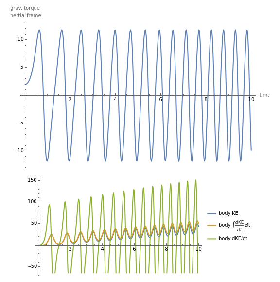
Notice the magnitude of the gravitational torque is not qualitatively what we’d expect. It should be zero when the pole is upright or dangling. On a swing-up arc, the torque should go through a “bounce” or “whiplash” as the sliding cart takes some of the lever arm away, thus have two maxima at zenith before falling.

The plots above show steadily increasing angular velocity and kinetic energy, plus a mismatch between kinetic energy and the integral of its derivative, which should always be equal.

But if I decrease

by a factor of 100 to 100 μsec, I get something much more sensible. It’s visibly not conservative over ten simulated seconds, but it shows the expected torque whiplash, plus the body KE and the integral of its derivative coincide within the resolution of the plot. This takes several minutes to run, so I save only a screenshot.

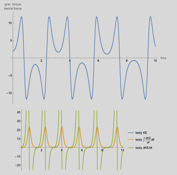
Conclusion:

The integrator is guilty.

Because decreasing the time increment results in physically plausible behavior and in better energy conservation, we deem the dynamics correct.

Stern-Desbrun Symplectic Integrator

◼

Section Abstract: This integrator produces plausible results for a small time step, but, in general, is too slow and unstable. We leave further investigation to the future, preferring to invest time in CGDVIE3. In particular, we have not profiled the code and we have not explored its poor energy conservation, which is supposed to be automatic via the discrete Noether’s Theorem. In the offing, for ground truth, we produce a good numerical integrator via Mathematica’s NDSolve. This integrator is not a primary objective of this work, but serves only to check others.

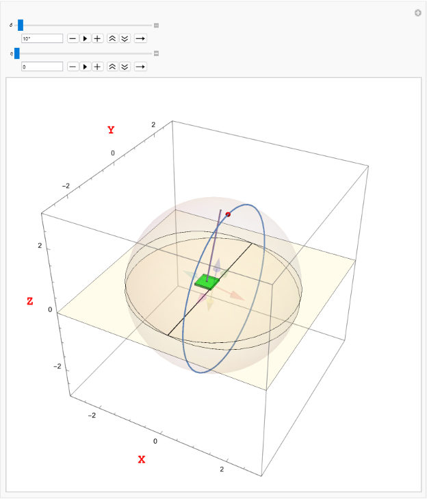
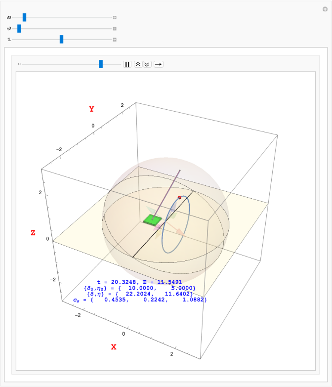
Recast the problem in Lagrangian form. What are good generalized coordinates and velocities of the pendulum? The obvious choice, spherical coordinates, has a singularity at the North pole, right where we want the baton to linger when get to controlling it. At the North pole, the longitude can be any number. A better choice of coordinates are pitch and an aerobatic, coordinated-cone roll (not axis roll!). These angles are co-latitude δ and an angular displacement η at a clockwise right angle to the great-circle arc of co-latitude. For any non-zero δ, spinning η makes a non-great circle on the surface around a pair of poles on the Equator. The demonstration below makes this visually clear. These poles are not as catastrophic as the North and South poles. Mathematica’s integrator produce interpolation functions that fly right through them. Both δ and η are zero at the North pole. η has two singularities on the Equator, when δ is 90° or 270°. But that situation is better than a singularity at the North pole because the baton will fly through these poles at the Equator, not linger at them.

The actual physical system is represented by the red ball at the center of mass of the baton, swinging around the origin. The sliding cart is a visual fiction, useful later when we control the baton. The Lagrangian, here, does not account for translational energy imparted by the cart, only rotational energy. We fix that later.

Demonstration of the Coordinate System

In[]:=

With[{epsilon=0.0001,h=1/15.,w=1/4.,vu=3.,o={0,0,0},thin={0,0,.0001},cb=rig["cb"]},With[{kart=Cuboid[{-w,-w,epsilon},{w,w,epsilon+h}],s=2,floor=Polygon[{{-vu,-vu,0},{vu,-vu,0},{vu,vu,0},{-vu,vu,0}}]},With[{c3=Cylinder[{o,thin},scb[[3]]],b3=Sphere[o,scb[[3]]],t3x=Tube[{-scb[[3]]e2,scb[[3]]e2},.01],axisLabelStyle=textStyle[text,Red,Bold,18,FontFamily"Courier New"]},Manipulate[DynamicModule[{renderPos=o,Στs=o,cs,rotfn},cs=RotationMatrix[-η,e1].RotationMatrix[δ,e2].cb;renderPos=-cs[[1]]e1-cs[[2]]e2;rotfn=RotationTransform[-η,e1]@*RotationTransform[δ,e2];Show[{Graphics3D[{GeometricTransformation[jack[0],rotfn],{Black,t3x},(*{White,Opacity[1./2],Cone[{RotationMatrix[δ,e2].cb,o},1]},*){White,Opacity[.7/8],c3,b3,GeometricTransformation[c3,RotationTransform[δ,e2]]},{Red,Sphere[scs,1/16.]},{Yellow,Opacity[.3/4],floor},{Green,Opacity[.6],Translate[kart,renderPos]},{White,Opacity[.75],Translate[Translate[GeometricTransformation[rig["graphics primitives"],rotfn],cs],renderPos+(epsilon+h)e3]}},ImageSizeLarge,AxesTrue,AxesLabelaxisLabelStyle/@{"X","Y","Z"},PlotRange{{-vu,vu},{-vu,vu},{-vu,vu}}],ParametricPlot3D[sRotationMatrix[-ha,e1].RotationMatrix[δ,e2].cb,{ha,0,2π}]}]],{{δ,10°},0°,360°,1°,Appearance->{"Open"}},{{η,0°},0°,360°,1°,Appearance->{"Open"}},SaveDefinitions->True]]]]

Out[]=

Dynamical Set-Up


Ground-Truth Solution with Initial Conditions

So we can check the Stern-Desbrun integrator later, let’s let Mathematica do its magical solution. We’ll regard that as ground truth. Even though it ends up pretty good, it’s not the end of the story because it’s opaque. We can’t easily see inside, so we can’t easily write a version in C or Python that does a good job. The Stern-Desbrun integrator, like our old RK4, is something we could code up in another programming language. That’s how we like to use Mathematica: as an executable design language for algorithms that we later code up in other programming languages for wider deployment.

Solve the system for

tLim=25

simulated seconds. Feel free to change this parameter. The solver is fast.

In[]:=

ClearAll[tLim,initialConditions,stSolns];tLim=25;initialConditions={δ[0]==10°,η[0]==5°,δ'[0]==0,η'[0]==0};stSolns=NDSolve[Append[stEqns,initialConditions]/.{

->1.2},{δ[t],η[t],δ'[t],η'[t]},{t,0,tLim}]

Out[]=

δ[t]InterpolatingFunction

Domain: {{0.,25.}}

Output: scalar

[t],η[t]InterpolatingFunction

Domain: {{0.,25.}}

Output: scalar

[t],

′

[t]InterpolatingFunction

Domain: {{0.,25.}}

Output: scalar

[t],

′

[t]InterpolatingFunction

Domain: {{0.,25.}}

Output: scalar

[t]

Plot the Solutions

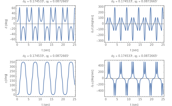
The solutions look pretty reasonable. I won’t go over all the physical intuitions in my nodding head. I consider the animation to be the most valuable validation that we’ve got this mostly right. More discussion follows the animation.

In[]:=

Manipulate[DynamicModule[{ics={δ[0]==δ0,η[0]==η0,δ'[0]==0,η'[0]==0},solns,δx,δDotx,ηx,ηDotx,flt},solns=NDSolve[Append[stEqns,ics]/.{

->1.2},{δ[t],η[t],δ'[t],η'[t]},{t,0,tL}];δx=solns[[1,1,2]];δDotx=solns[[1,3,2]];ηx=solns[[1,2,2]];ηDotx=solns[[1,4,2]];flt="

= "<>ToString[δ0]<>"°,

= "<>ToString[η0]<>"°";GraphicsGrid[{{Plot[δx/°,{t,0,tL},FrameLabel->{{"δ [deg]",""},{"t [sec]",flt}},Frame->True],Plot[δDotx/°,{t,0,tL},FrameLabel->{{"

∂

δ [deg/sec]",""},{"t [sec]",flt}},Frame->True]},{Plot[ηx/°,{t,0,tL},FrameLabel->{{"η [deg]",""},{"t [sec]",flt}},Frame->True],Plot[ηDotx/°,{t,0,tL},FrameLabel->{{"

∂

η [deg/sec]",""},{"t [sec]",flt}},Frame->True]}}]],{{δ0,10.°},0.,90.°},{{η0,5.°},0,90.°},{{tL,25},0,50},SaveDefinitions->True]

Out[]=

δ0

η0

Phase Portrait

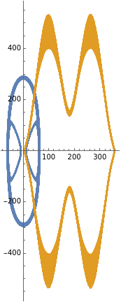
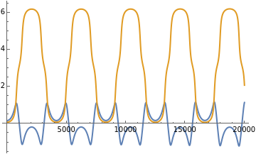
Plot the angles versus their velocities, proportional to their Hamiltonian conjugate momenta. If the solution were conservative, these phase portraits would be thin lines. When the time constant is long (400 seconds, here), however, they thicken up, showing that the solution is slightly non-conservative, but it’s much better than our RK4 on Quaternions. This is going to be a good ground-truth.

In[]:=

Manipulate[DynamicModule[{ics={δ[0]==δ0,η[0]==η0,δ'[0]==0,η'[0]==0},solns,δx,δDotx,ηx,ηDotx},solns=NDSolve[Append[stEqns,ics]/.{

->1.2},{δ[t],η[t],δ'[t],η'[t]},{t,0,tL}];δx=solns[[1,1,2]];δDotx=solns[[1,3,2]];ηx=solns[[1,2,2]];ηDotx=solns[[1,4,2]];ParametricPlot[{{δx,δDotx}/°,{ηx,ηDotx}/°},{t,0,tL},PlotLegends->{"δ","η"}]],{{δ0,10.°},0,90.°},{{η0,5°},0,90.°},{{tL,400},0,500},SaveDefinitions->True]

Out[]=

δ0

η0

	δ
	η

Ground-Truth Animation

This is pretty convincing. Energy is well conserved. If we were satisfied with an integrator that works only inside Mathematica, we’d be just about done. But we want an integrator we can code up in any programming language. Next stop is to do as well with a discrete Stern-Desbrun integrator, but we’ll find that difficult.

In[]:=

With[{epsilon=0.0001,h=1/15.,w=1/4.,vu=3.},With[{ztxt=-1.5,xtxt=0,ytxt=-2,znl=0.3},With[{kart=Cuboid[{-w,-w,epsilon},{w,w,epsilon+h}],floor=Polygon[{{-vu,-vu,0},{vu,-vu,0},{vu,vu,0},{-vu,vu,0}}],axisLabelStyle=textStyle[text,Red,Bold,18,FontFamily"Courier New"],cb=rig["cb"],thin={0,0,.0001},s=2,o={0,0,0}},With[{c3=Cylinder[{o,thin},scb[[3]]],b3=Sphere[o,scb[[3]]],t3x=Tube[{-scb[[3]]e2,scb[[3]]e2},.01]},Manipulate[DynamicModule[{ics={δ[0]==δ0,η[0]==η0,δ'[0]==0,η'[0]==0},solns,δx,Dδx,ηx,Dηx,flt},

solns=NDSolve[Append[stEqns,ics]/.{

->1.2},{δ[t],η[t],δ'[t],η'[t]},{t,0,tL}]

;δx=solns[[1,1,2]];Dδx=solns[[1,3,2]];ηx=solns[[1,2,2]];Dηx=solns[[1,4,2]];Animate[Module[{renderPos=o,cs,rotfn},cs=RotationMatrix[-ηx/.t->u,e1].RotationMatrix[δx/.t->u,e2].cb;renderPos=-cs[[1]]e1-cs[[2]]e2;rotfn=RotationTransform[-ηx/.t->u,e1]@*RotationTransform[δx/.t->u,e2];Show[{Graphics3D[{Text[font["t = "<>nfm@u<>", E = "<>nfm@(Tnum[{δx/.t->u,ηx/.t->u},{Dδx/.t->u,Dηx/.t->u}]+Vnum[{δx/.t->u,ηx/.t->u}])],{xtxt,ytxt,ztxt}],Text[font["{

} = "<>vfm@{δ0/°,η0/°}],{xtxt,ytxt,ztxt-znl}],Text[font["{δ,η} = "<>vfm@{(δx/.t->u)/°,(ηx/.t->u)/°}],{xtxt,ytxt,ztxt-2znl}],Text[font["

= "<>vfm@cs],{xtxt,ytxt,ztxt-3znl}],{Black,t3x},{White,Opacity[.7/8],c3,b3,GeometricTransformation[c3,RotationTransform[δx/.t->u,e2]]},GeometricTransformation[jack[0],rotfn],{Red,Sphere[cs,1/16.]},{Yellow,Opacity[.3/4],floor},{Green,Opacity[.6],Translate[kart,renderPos]},{White,Opacity[.75],Translate[Translate[GeometricTransformation[rig["graphics primitives"],rotfn],cs],renderPos+(epsilon+h)e3]}},ImageSizeLarge,AxesTrue,AxesLabelaxisLabelStyle/@{"X","Y","Z"},PlotRange{{-vu,vu},{-vu,vu},{-vu,vu}}],ParametricPlot3D[RotationMatrix[-ha,e1].RotationMatrix[δx/.t->u,e2].cb,{ha,0,2π}]}]],{u,0,tL},AnimationRate->.5]],{{δ0,10.°},0,90.°},{{η0,5.°},0,90.°},{{tL,25},0,50},SaveDefinitions->True]]]]]

Out[]=

Discrete Lagrangian

Instead of integrating those equations, let’s discretize the Lagrangian, itself, via Equation 7 of Reference 10. First, a reminder

In[]:=

??Lnum

Out[]=

Symbol

Global`Lnum

Definitions

Lnum[{δ_,η_},{Dδ_,Dη_}]:=Tnum[{δ,η},{Dδ,Dη}]-Vnum[{δ,η}]

Full Name

Global`Lnum

Whereas LNum takes a coordinate tuple q and a velocity tuple



, the poorly named discrete Lagrangian

takes a pair of coordinate tuples: one,

, at time

and another,

k+1

, at time

k+1

is poorly named because it’s actually an increment of action (units of energy × time), being the product of a value of LNum (units of energy) and the finite (constant) time increment dt (

in the paper). Despite the notation in the paper,

depends on

. We capture that dependence in our rendition of

. Despite the fact that

is a constant, for now, we might want to vary it later. We assume midpoint quadrature, halfway between

and

k+1

In[]:=

ClearAll[Ld,pk,pkp1,δkm1,ηkm1,δk,ηk,δkp1,ηkp1,dt];Ld[qk:{δk_,ηk_},qkp1:{δkp1_,ηkp1_},dt_]:=dtLnum

(qk+qkp1),

(qkp1-qk);

Discrete Euler-Lagrange Equations

The discrete Euler-Lagrange equations (DELE) are

(

k+1

(

k-1

)=0

(

)

As Stern and Desbrun point out, DELE imply a recurrence, automatically suitable for an integrator. I go a tiny step further and note that it’s almost a foldable as it stands. We’ll use that fact to advantage shortly. A wrinkle is that DELE require two initial positions (δ-η tuples), whereas we have initial positions and velocities. There is enough information to get two initial positions, however, via a numerical root in the position-momentum form shown in Section 5.3 of Reference 10.

First, we need the derivatives.

({

},{

k+1

})=

∂

(...),

∂

(...)

and

({

},{

k+1

})=

∂

k+1

(...),

∂

k+1

(...)

. Mathematica’s Evaluate in Place is handy for this, because we only need the symbolic derivatives once. Here are closed forms for the conjugate momenta

and

k+1

via Equation 8 of Reference 10.

In[]:=

pk[{δk_,ηk_},{δkp1_,ηkp1_},dt_]:=(*-

(

k+1

)*)(*-{D[Ld[{δk,ηk},{δkp1,ηkp1},dt],δk]//FullSimplify,D[Ld[{δk,ηk},{δkp1,ηkp1},dt],ηk]//FullSimplify},EvaluateinPlace*)-

-1.44(-δk+δkp1)+5.886

Cos

ηk+ηkp1

Sin

δk+δkp1

-0.36

(ηk-ηkp1)

Sin[δk+δkp1]

0.72ηk-0.72ηkp1+(0.72ηk-0.72ηkp1)Cos[δk+δkp1]+5.886

Cos

δk+δkp1

Sin

ηk+ηkp1



;pkp1[{δk_,ηk_},{δkp1_,ηkp1_},dt_]:=(*+

(

k+1

)*)(*+{D[Ld[{δk,ηk},{δkp1,ηkp1},dt],δkp1]//FullSimplify,D[Ld[{δk,ηk},{δkp1,ηkp1},dt],ηkp1]//FullSimplify},EvaluateinPlace*)

1.44(-δk+δkp1)+5.886

Cos

ηk+ηkp1

Sin

δk+δkp1

-0.36

(ηk-ηkp1)

Sin[δk+δkp1]

-0.72ηk+0.72ηkp1+(-0.72ηk+0.72ηkp1)Cos[δk+δkp1]+5.886

Cos

δk+δkp1

Sin

ηk+ηkp1



;

Visual Sanity Check

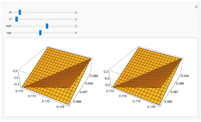
Plot momentum surfaces for a manipulable interval

±b

around the manipulable initial conditions

=10°

and

=5°

that we had in the ground truth default. We’re looking to see that the zeros of these momenta are in range, because they imply the second position initials,

and

In[]:=

ManipulateWith{b=

logb

10.

},GraphicsRowPlot3Dpk{δ0,η0},{δ1,η1},

logdt

10.

,{δ1,δ0-b,δ0+b},{η1,η0-b,η0+b},Plot3Dpkp1{δ0,η0},{δ1,η1},

logdt

10.

,{δ1,δ0-b,δ0+b},{η1,η0-b,η0+b},{{δ0,10.°},0,90.°},{{η0,5.°},0,90.°},{{logdt,-2.},-6,1},{{logb,Log10[.1°]},Log10[0.0001°],Log10[360°]},SaveDefinitions->True

Numerical Solution for
δ
1
and
η
1

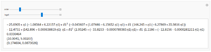
The equations are too hard to solve symbolically, so we suffice with a numerical solution of series expansions of the trigonometric functions. The following experiment shows that order-2 solutions, with a little safety margin, at

dt=0.01

are fast enough and good enough to get started.

In[]:=

With{b=10.°,δ0=10.°,η0=5.°,pδ0=0.0,pη0=0.0},ManipulateWith{dt0=

logdt

},With[{ps1=Normal[Series[pk[{δ0,η0},{δ1,η1},dt0][[1]],{δ1,δ0,order},{η1,η0,order}]],ps2=Normal[Series[pk[{δ0,η0},{δ1,η1},dt0][[2]],{δ1,δ0,order},{η1,η0,order}]]},With[{radians=AbsoluteTiming@NSolve[ps1==pδ0&&ps2==pη0&&Abs[δ0-δ1]<b&&Abs[η0-η1]<b,{δ1,η1},Reals]},Column[{ps1//FullSimplify,ps2//FullSimplify,radians[[1]],{radians[[2,1,1,2]],radians[[2,1,2,2]]}/N[°],{radians[[2,1,1,2]],radians[[2,1,2,2]]}}]]],{{order,2},1,6,1},{{logdt,-2},-6,0,1},SaveDefinitions->True

bootIntegrator

Package the solution in a function so we can call it to bootstrap the integrator.

In[]:=

ClearAll[bootIntegrator];

bootIntegrator[b_,δ0_,η0_,pδ0_,pη0_,logdt_:-2,order_:2]

:=With{dt0=

logdt

Out[]=

Solve

(

k+1

k+2

(

k+1

)==0

for

k+2

when

k>=0

. Reuse functions pk and pkp1 from above, by advancing pk one step. Sneak in non-conservative forces for the right-hand side of the Equation 7 of Reference 10, looking forward to the future. Sanity check: expect δ and η to increase a little as the baton falls.

In[]:=

(*-pk[{δkp1_,ηkp1_},{δkp2_,ηkp2_},dt_]:=

(

k+1

k+2

)*)(*pkp1[{δk_,ηk_},{δkp1_,ηkp1_},dt_]:=

(

k+1

)*)

In[]:=

With[{b=10.°,δ0=10.°,η0=5.°,pδ0=0.0,pη0=0.0,dt0=0.01,order=2,forces=0},With[{q1=bootIntegrator[b,δ0,η0,pδ0,pη0]},(*numerical*)With[{δk=δ0,ηk=η0,δkp1=q1[[1,1,2]],ηkp1=q1[[1,2,2]]},(*bootstrap*)Module[{δkp2,ηkp2},With[{dele=pkp1[{δk,ηk},{δkp1,ηkp1},dt0]-pk[{δkp1,ηkp1},{δkp2,ηkp2},dt0]},With[{solns=NSolve[Normal[Series[dele,{δkp2,δkp1,order},{ηkp2,ηkp1,order}]]==forces&&Abs[δkp2-δkp1]<b&&Abs[ηkp1-ηkp2]<b,{δkp2,ηkp2},Reals]},Column[{{δkp1,ηkp1},{solns[[1,1,2]],solns[[1,2,2]]}}]]]]]]]

Out[]=

{0.174604,0.0873026}

{0.174816,0.0874112}

Package the solver as a foldable and run it for a while. I had to reduce the time step to 1.25 msec to get plausible results. It takes too long, so I saved only a screen shot. It eventually goes wild, so we move on: too slow and not sufficiently conservative. The following cell is not evaluatable. Change it via Mathematica’s Cell menu if you want to devote some time to playing around with it.

ClearAll[foldableDele];With[{b=10.°,δ0=10.°,η0=5.°,pδ0=0.0,pη0=0.0},With[{q1=bootIntegrator[b,δ0,η0,pδ0,pη0]},(*numerical*)

foldableDele[{{δk_,ηk_},{δkp1_,ηkp1_}},tkp1_]

:=With[{order=2,forces=0},Module[{δkp2,ηkp2},With[{dele=pkp1[{δk,ηk},{δkp1,ηkp1},tkp1]-pk[{δkp1,ηkp1},{δkp2,ηkp2},tkp1]},With[{solns=NSolve[Normal[Series[dele,{δkp2,δkp1,order},{ηkp2,ηkp1,order}]]==forces&&Abs[δkp2-δkp1]<b&&Abs[ηkp1-ηkp2]<b,{δkp2,ηkp2},Reals,WorkingPrecision->24]},{{δkp1,ηkp1},{solns[[1,1,2]],solns[[1,2,2]]}}]]]];With[{tL=20000,dt0=0.00125},With[{qs=Quiet@FoldList[foldableDele,{{δ0,η0},{q1[[1,1,2]],q1[[1,2,2]]}},ConstantArray[dt0,tL]]},qs;ListLinePlot[{#[[2,1]]&/@qs,#[[2,2]]&/@qs}]]]]]

Out[]=

Conclusion: we leave further investigation of this solver to the future. In particular, we have not explored its energy conservation, purportedly automatic, but manifestly not.

DREPE, DRNEA, and CGDVIE3

Go back to quaternions, and from there to the group SE(3).[4] We’ll integrate directly on the manifold of SE(3) via discrete methods. We’ll bring up Dzhanybekhov, 4DISP in a later notebook.

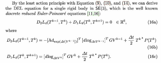
There is a lot of machinery, here. It’s mostly about implementing Equations 16b and 16c in Reference 2. Notice that Equation 16a is exactly the same as we have above in DEL, but in a 6-dimensional coordinate system on SE(3) instead of in our 2-dimensional Lagrangian coordinate system. These equations contain an undefined term,

. I have contacted the authors to find out what it might be. I suspect it to be an adjoint representation of a force in the co-tangent bundle, but getting this right will require more research.

Out[]=

Utilities


Proofs and Tests

Conceptual Checks

Test the effects of frame rotations of yaw, pitch, and roll on the axes of the BODY FRAME.

Consider

, pointing in the positive

direction of the body, that is, NORTH. After a small yaw, we expect this vector to have a small, positive

component, a zero

component, and an

component less than 1.

To turn

into a column vector, all we have to do is map List over it.

In[]:=

R

N@Pi

,0,0.(List/@e1)//MatrixForm

Out[]//MatrixForm=

0.965926

0.258819

Looks good!

After a small pitch, we expect

to have a small, negative

component (that is, up), a zero

component, and an

component less than 1.

In[]:=

R0,

N@Pi

,0.(List/@e1)//MatrixForm

Out[]//MatrixForm=

0.965926

-0.258819

Good!

Roll should not affect

In[]:=

R0,0,

N@Pi

.(List/@e1)//MatrixForm

Out[]//MatrixForm=

Expect yaw to give

a small, negative

component, a reduced

component, and a zero

component:

In[]:=

R

N@Pi

,0,0.(List/@e2)//MatrixForm

Out[]//MatrixForm=

-0.258819

0.965926

Expect pitch to leave

unchanged:

In[]:=

R0,

N@Pi

,0.(List/@e2)//MatrixForm

Out[]//MatrixForm=

Expect roll to give

a small, positive

component (that is, down), a reduced

component, and to leave the

component unchanged:

In[]:=

R0,0,

N@Pi

.(List/@e2)//MatrixForm

Out[]//MatrixForm=

0.965926

0.258819

Yaw should not affect

In[]:=

R

N@Pi

,0,0.(List/@e3)//MatrixForm

Out[]//MatrixForm=

Pitching

up should yield a small, positive

component, a reduced

component, and should leave

unchanged:

In[]:=

R0,

N@Pi

,0.(List/@e3)//MatrixForm

Out[]//MatrixForm=

0.258819

0.965926

Rolling

should yield a small, negative

component, a reduced

component, and an unchanged

component:

In[]:=

R0,0,

N@Pi

.(List/@e3)//MatrixForm

Out[]//MatrixForm=

-0.258819

0.965926

Investigate Formulae

In[]:=

<<Notation`QuietSymbolize

;Symbolize

;

In[]:=

shorteningRules={Cos[x_]

,Sin[y_]

};

In[]:=

lengtheningRules={

Cos[x],

Sin[y]};

In[]:=

R[ψ,θ,ϕ]/.shorteningRules//MatrixForm

Out[]//MatrixForm=

c θ c ψ	- c θ s ψ	s θ
c ψ s θ s ϕ + c ϕ s ψ	c ϕ c ψ - s θ s ϕ s ψ	- c θ s ϕ
- c ϕ c ψ s θ + s ϕ s ψ	c ψ s ϕ + c ϕ s θ s ψ	c θ c ϕ

For verifying frame rotation, it’s best to reverse the signs of all angles. This next one matches Guangyu Liu’s dissertation on the inverted, spherical pendulum, his Equation 2.8:

In[]:=

R[-ψ,-θ,-ϕ]/.shorteningRules//MatrixForm

Out[]//MatrixForm=

c θ c ψ	c θ s ψ	- s θ
c ψ s θ s ϕ - c ϕ s ψ	c ϕ c ψ + s θ s ϕ s ψ	c θ s ϕ
c ϕ c ψ s θ + s ϕ s ψ	- c ψ s ϕ + c ϕ s θ s ψ	c θ c ϕ

This is not the same as the transpose of

R[ψ,θ,ϕ]

In[]:=

R[ψ,θ,ϕ]/.shorteningRules//MatrixForm

Out[]//MatrixForm=

c θ c ψ	c ψ s θ s ϕ + c ϕ s ψ	- c ϕ c ψ s θ + s ϕ s ψ
- c θ s ψ	c ϕ c ψ - s θ s ϕ s ψ	c ψ s ϕ + c ϕ s θ s ψ
s θ	- c θ s ϕ	c θ c ϕ

but that, of course, is the same as the product of the transposes of the composed matrices, in opposite order:

In[]:=

RotationMatrix[ψ,e3].RotationMatrix[θ,e2].RotationMatrix[ϕ,e1]/.shorteningRules//MatrixForm

Out[]//MatrixForm=

c θ c ψ	c ψ s θ s ϕ + c ϕ s ψ	- c ϕ c ψ s θ + s ϕ s ψ
- c θ s ψ	c ϕ c ψ - s θ s ϕ s ψ	c ψ s ϕ + c ϕ s θ s ψ
s θ	- c θ s ϕ	c θ c ϕ

What is Liu up to?

In the following demonstration, the first and last images should be always the same. The second and third images are for inspection.

In[]:=

With[{rg={-1.5,1.5}},Manipulate[GraphicsGrid[{{Graphics3D[GeometricTransformation[jack[rq0,1.0],

R[ψ,θ,ϕ]

],PlotRange{rg,rg,rg},ImageSizeMedium],Graphics3D[GeometricTransformation[jack[rq0,1.0],

R[ψ,θ,ϕ]

],PlotRange{rg,rg,rg},ImageSizeMedium],Graphics3D[GeometricTransformation[jack[rq0,1.0],

R[-ψ,-θ,-ϕ]

],PlotRange{rg,rg,rg},ImageSizeMedium]},{Graphics3D[GeometricTransformation[jack[rq0,1.0],

RollPitchYawMatrix[{ψ,θ,ϕ}]

],PlotRange{rg,rg,rg},ImageSizeMedium]}}],{{ψ,0},0,2Pi,Appearance"Labeled"},{{θ,0},0,2Pi,Appearance"Labeled"},{{ϕ,0},0,2Pi,Appearance"Labeled"},SaveDefinitions->True]]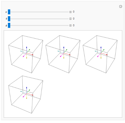

Our

matrix is algebraically identical to Mathematica’s built-in:

In[]:=

R[ψ,θ,ϕ]===RollPitchYawMatrix[{ψ,θ,ϕ}]

Out[]=

True

Another proof:

These two forms are algebraically equal, at least according to Mathematica, which cancels divisors without stipulation that they be non-zero. Because of that feature, we also need the numerical work above.

In[]:=

R[ψ,θ,ϕ].

rvQ[ψ,θ,ϕ],

//FullSimplify

Out[]=

True

DREPE, DRNEA, and CGDVIE3 Theory


DRNEA (Reference 2)

SO(3), (3)

Definitions

SO(3) is the set of

3×3

orthogonal matrices with unit determinant

(no reflections). Its Lie algebra is the set (3) of

3×3

skew-symmetric matrices

such that the matrix exponential



is in SO(3). The notation

is clarified below.

Quoting reference [6]:

◼

Definition 3.18. “Let

be a matrix Lie group. The Lie algebra of

, denoted , is the set of all matrices

such that



is in

for all real numbers

.”

The definition gives us a way to generate an element of

from any element

of . Does it go the other way? Can we recover



∈G

from an element

of  ?

Assume we can. Write an element of

g∈G



. The formal derivative of



, evaluated at

t=0

, namely



t=0

, recovers

. Generalize: find a one-variable parameterization of the Lie group, differentiate

g(t)

with respect to the one parameter

, and evaluate the derivative at

t=0

The recovered element

X∈

is unique, but, typically, many elements in the Lie algebra  map to the same element

in the Lie group, as we show below.

Example

Let

G=SO(3)

, rotation matrices in Euclidean 3-space. Here is a yaw-only object-rotation matrix in SO(3):

In[]:=

R[ψ,0,0]//MatrixForm

Out[]//MatrixForm=

Cos[ψ]	-Sin[ψ]	0
Sin[ψ]	Cos[ψ]	0
0	0	1

By hypothesis, it corresponds to some as-yet-unknown element

of the Lie algebra (3). Identify the parameter

of the curve



with ψ and evaluate the derivative:

In[]:=

D[R[ψ,0,0],ψ]//MatrixForm

Out[]//MatrixForm=

-Sin[ψ]	-Cos[ψ]	0
Cos[ψ]	-Sin[ψ]	0
0	0	0

Evaluate at

t=ψ=0

In[]:=

Gso33=D[R[ψ,0,0],ψ]/.{ψ0}//MatrixForm

Out[]//MatrixForm=

0	-1	0
1	0	0
0	0	0

That’s one generator or basis element of (3). Here are the other two, by the same procedure on the other two angles, namely pitch

and roll

In[]:=

Gso32=D[R[0,θ,0],θ]/.{θ0}//MatrixForm

Out[]//MatrixForm=

0	0	1
0	0	0
-1	0	0

In[]:=

Gso31=D[R[0,0,ϕ],ϕ]/.{ϕ0}//MatrixForm

Out[]//MatrixForm=

0	0	0
0	0	-1
0	1	0

Given the basis matrices above, we can form all skew-symmetric matrices by linear combinations:

(1)

(3)

(2)

(3)

(3)

(3)

;

∈,i∈[1..3]

It is convenient to say that the Lie algebra is this large set of all skew-symmetric matrices. However, some of those skew-symmetric matrices map to the same rotations, as demonstrated below. The mapping from this Lie algebra to its Lie group is many-to-one, and the inverse mapping either doesn’t exist (to a mathematician) or is multi-valued (to a physicist), requiring a particular choice to produce a single value.

Naming Convention (Hungarian Types)

We write reminders of the types of variables and of the output types of functions as suffixes like So3 or so3 for (3), R3 for



, SO3 for SO(3), and so on. For example, hatSo3 returns an element of (3), taking an element of



as input. unHatR3 returns an element of



, taking an element of SO(3) as input. We don’t write reminders of input types; remember them or look them up. To ease the cognitive load, we provide convenience overloads based on Mathematica pattern-matching. We may write an overload that automatically senses the input types you want. For example, we have TSE3[ψ,θ,ϕ,x,y,z] and also TSE3[Quat[w,ix,jy,kz],{x,y,z}]. The former takes yaw, pitch, roll angles and three Cartesian displacements. The latter takes a rotation quaternion and a list of Cartesian displacement. They both return elements of SE(3), that is, properly formatted

4×4

matrices.

The type of

6×6

matrices is 6R6. The type of

6×1

column vectors is 6R1. The type of

1×6

row vectors is 1R6. The type of a

2×3

matrix is 2R3, and so on. The type of a flat list or vector with 6 elements is R6.

Ideally, types would contain units-of-measure, but such would lead to excessively long reminders, and not work at all for matrices that contain elements with different units-of-measure. For now, we live with shape types (e.g., 6R6) and domain types (e.g., SO(3)). See https://math.stackexchange.com/questions/1275724/when-should-matrices-have-units-of-measurement and Multidimensional Analysis (https://a.co/d/8c5RqOX).

We tend to camel-case, where the first character in a name is lower-case and intermediate sub-names are capitalized. However, due to the many capital letters in the mathematical references, due to ambiguity about whether or how to capitalize after a fully capitalized acronym, and due to ambiguity about whether to capitalize after numerals, we admit to inconsistency in this convention.

Names that begin with dollar signs are Mathematica built-ins, like $MachineEpsilon = 2.2204*^-16. Names that end with dollar signs signify ad-hoc variables, that is, mutable variables. Names without dollar signs at the end may be trusted to have the same meanings everywhere in the document, but names with dollar signs at the ends, such as T0$, T1$, and T2$, may not be so trusted. We feel free to change their meanings at will to serve some purpose near-at-hand.

Vectors as Lists, Column Vectors, Row Vectors

Mathematica and Python share the feature that vectors are sometimes just flat lists and sometimes are lists of lists, that is,

n×1

matrices — column vectors, or

1×n

matrices — row vectors. Many operations, like dot products, work whether you give them a list or a list of lists. But some operations, like Transpose, are only meaningful on lists of lists. This intentional ambiguity is intentionally risky, but we live with it for now.

hatSo3:
3

(3)
, unHatR3:
(3)
3


An element of (3) is any skew-symmetric matrix

. The subscript × means “skew symmetric” and should evoke 3D cross product in your mind. Such a matrix has only three independent elements, so it corresponds bijectively to an element of



. The hat map is invertible; it just rearranges components from a vector ω in



into a matrix

. The inverse map unHat moves the elements of back into a vector ω. Both directions are total, meaning that every

ω∈



corresponds to an element of (3), and vice versa.

In[]:=

ClearAll[hatSo3,unHatR3];hatSo3[ω1_,ω2_,ω3_]:=

0	-ω3	ω2
ω3	0	-ω1
-ω2	ω1	0

;(*Convenienceoverload,takingavector-as-list;theotherconvenienceoverloads,takingavector-as-column-vectorwillbeintroducedifneeded(TODO).*)hatSo3[{ω1_,ω2_,ω3_}]:=hatSo3[ω1,ω2,ω3];unHatR3[ωHat_]:={ωHat[[3,2]],-ωHat[[3,1]],ωHat[[2,1]]};

The square of hat appears below in Rodrigues’ formula.

In[]:=

hatSo3[ω1,ω2,ω3].hatSo3[ω1,ω2,ω3]//MatrixForm

Out[]//MatrixForm=

- 2 ω2 - 2 ω3	ω1ω2	ω1ω3
ω1ω2	- 2 ω1 - 2 ω3	ω2ω3
ω1ω3	ω2ω3	- 2 ω1 - 2 ω2

◼

Unit Test

In[]:=

With[{ωx=hatSo3[ω1,ω2,ω3]},unHatR3[ωx]]

Out[]=

{ω1,ω2,ω3}

expSO3:
(3)SO(3)
, AKA Rodrigues’ Formula

◼

“Rodrigues’” is spelled with no “s” after the possessive apostrophe at the end because the last “s” in “Rodrigues” is voiced. There is no consensus for such punctuation, but this is the way AMS [American Mathematical Society] does it. APA [American Psychological Association] would have us write “Rodrigues’s.”

Rodrigues’ formula (https://en.wikipedia.org/wiki/Rodrigues%27_rotation_formula) remarkably presages Lie theory by some decades.

The following version of the exp map is not suitable for symbolic computations because it has a numerical test for small angles. We factor out the small-angle computations because we need them later for SE(3) and (3). We make a symbolic version later below.

◼

θThresh: Global Constant

When angles are smaller than θThresh, functions use an explicit Taylor series rather than built-ins to prevent division by small floating-point numbers.

Truncate all series in the angular variable θ at the eighth degree because 0.01 to the eighth power is

-16

, at or near the precision of double-precision floating-point numbers, and we use 0.01 frequently as a discrete increment. In this sense, all our series “know” that the threshold for transitioning from built-in functions to explicit Taylor series is 0.01. We do not expect this “knowledge leak” to be trouble, but we may need to keep any eye out for it.

In[]:=

ClearAll[θThresh];θThresh=0.01;(*

≈$MachineEpsilon*)

◼

sθOverθ: Sin[θ]/θ

In[]:=

ClearAll[sθOverθ];sθOverθ[θ_]:=Ifθ<θThresh,(*

≈$MachineEpsilon*)1-

,(*Series

Sin[θ]

,{θ,0,9}*)

Sin[θ]

;

◼

oneMcθOverθ2:

(1-Cos[θ])/

In[]:=

ClearAll[oneMcθOverθ2];oneMcθOverθ2[θ_]:=Ifθ<θThresh,

10!

1-Cos[θ]

;(*Series

1-Cos[θ]

,{θ,0,9}*)

◼

expSO3:



In[]:=

ClearAll[expSO3];expSO3[ωHat_]:=With[{ω=unHatR3[ωHat]},With[{θ=Sqrt[ω.ω]},With[{c1=sθOverθ[θ],c2=oneMcθOverθ2[θ]},IdentityMatrix[3]+c1ωHat+c2ωHat.ωHat]]];

The expression

exp[

]=I+

Sin[θ]

1-Cos[θ]

,withθ=

(

)

is Rodrigues’ rotation formula when the norm (Euclidean length) of

is equal to the angle of twist. Many other derivations of Rodrigues’ formula assume ω is a unit vector and present

exp[θω]

, resulting in no denominators in the coefficients. Getting rid of denominators might reduce the need for explicit series and therefore the risk of truncation error (TODO: consider rewriting all the code without denominators).

logSo3:
SO(3)(3)

log takes us back to a canonical member of (3) on the principal branch.

◼

θOver2sθ:

θ/(2Sin[θ])

In[]:=

ClearAll[θOver2sθ];θOver2sθ[θ_]:=Ifθ<θThresh,

720

30240

127

1209600

,(*https://dlmf.nist.gov4.19.4,http://oeis.orgA036280,http://oeis.orgA036281,Series

2Sin[θ]

,{θ,0,9}*)

2Sin[θ]

;

◼

logSo3

In[]:=

ClearAll[logSo3];logSo3[R_]:=Withθ=ArcCos

(Tr[R]-1),(R-R)*θOver2sθ[θ];

◼

Unit Test

Numerically, log and exp round trip to a part in

almost all the time. It fails occasionally at one part in

, frequently enough that the following test of

10000

trials will usually not succeed if rounders is

-7

. Because logSo3 canonicalizes

, we must compare results in SO(3) and not in (3).

In[]:=

SelectTableWithbig=10.0,rounder=

-6

,With[{ω=RandomReal[{-big,big},3]},With[{RSO3=expSO3[hatSo3[ω]]},With[{R2SO3=expSO3[logSo3[RSO3]]},With[{lhs=N@Round[RSO3,rounder],rhs=N@Round[R2SO3,rounder]},lhsrhs]]]],10000,#False&//Length

Out[]=

◼

logSo3symbolic

For some purposes, we need an exact, or symbolic, version of logSo3:

In[]:=

ClearAll[logSo3symbolic];logSo3symbolic[R_]:=Withθ=ArcCos

(Tr[R]-1),(R-R)*

2Sin[θ]

;

Remarks

Multiplication in the reals is commutative; log on the reals converts a commutative product into a commutative sum. We might wish for something similar with rotation matrices, but it cannot be. Matrix products do not commute, but sums do. The log of

cannot, in general, equal the log of

. What is the log of a product of rotation matrices? The answer is in an application of the Baker-Campbell-Hausdorff formula.[11-13] This is non-trivial but not immediately needed in the current work.

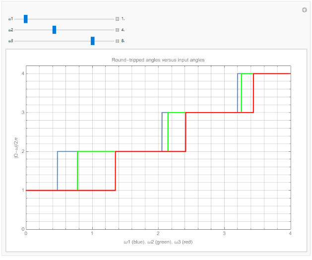
Geometrically,

ω≡

is an axis-angle vector. Its direction specifies the axis about which a twist occurs, and its length specifies the counterclockwise angle of twist in radians. Many different twist vectors map to the same rotation matrix. In the following demonstration, you may choose components for ω varying from 0 through some big number, and three sweeps are shown in red, green, and blue. Each sweep shows the difference in Norm (Euclidean length or magnitude) in units of

2π

, between your chosen ω and unhat[log[exp[hat[ω]]]], which latter specifies a canonical choice for the same rotation. Each sweep covers one of the three components, the other two being fixed by your interactive choices. This demonstration illustrates that unhat[log[exp[hat[ω]]] finds a the shortest twist vector (of smallest norm) that specifies the same rotation as the original choice, subtracting the maximum allowable multiples of

2π

along the original direction of ω.

In[]:=

With[{big=10.,maxsweep=4,unit=2π},Manipulate[With[{ω={ω1,ω2,ω3},uleh=unHatR3@*logSo3@*expSO3@*hatSo3,klugh={Ω,ω}(Norm[Ω-ω]/unit)},Grid[{{Show[{Plot[klugh[{w1*unit,ω2,ω3},uleh[{w1*unit,ω2,ω3}]],{w1,0,maxsweep},GridLinesFull,FrameTrue,FrameLabel{{"|Ω-ω|/2π",""},{"ω1 (blue), ω2 (green), ω3 (red)","Round-tripped angles versus input angles"}},ImageSizeLarge,PlotRange{{0,maxsweep},{0,1.05maxsweep}}],Plot[klugh[{ω1,w2*unit,ω3},uleh[{ω1,w2*unit,ω3}]],{w2,0,maxsweep},ColorFunction(Green&)],Plot[klugh[{ω1,ω2,w3*unit},uleh[{ω1,ω2,w3*unit}]],{w3,0,maxsweep},ColorFunction(Red&)]}],SpanFromLeft}}]],{{ω1,.10*big},0,big,Appearance"Labeled"},{{ω2,.4*big},0,big,Appearance"Labeled"},{{ω3,.8*big},0,big,Appearance"Labeled"},SaveDefinitions->True]]

Just as the exponential map from

θ∈(2)

to SO(2),

iθ

=cosθ+isinθ

, maps many angles to the same complex-number “rotator,” the exponential map from

∈(3)

to SO(3) maps many

to the same rotation matrix. The log or pseudoinverse-exp map “unwinds” multiples of

2π

on its principal branch. Similarly, from SO(2), the log or inverse-exp map is ArcTan, which also requires a choice of principal branch.

Adjoint in SO(3)

The adjoint

Adj

of element

of SO(3) is another

3×3

matrix defined by the equation

exp[

(

Adj

·ω)

]=R·exp[

]·R

(

)

ω is a three-vector inside the left-hand side and the skew-symmetric hat form

appears inside the right-hand side. The right-hand side’s expression is a matrix product, obviously in SO(3) because all its factors are in SO(3).

◼

Unit Tests

Reference [4] asserts that the adjoint of

in SO(3) is just

again. Check this assertion.

As noted above, we need a symbolic version of the exp map from (3) to SO(3).

In[]:=

ClearAll[expSO3symbolic];expSO3symbolic[ωHat_]:=With{ω=unHatR3[ωHat]},With{θ=Sqrt[ω.ω]},(*punningrowandcolumnvectorsaslists*)IdentityMatrix[3]+

Sin[θ]

ωHat+

1-Cos[θ]

ωHat.ωHat

The “theta” for pitch in our general rotation matrix is different from the θ in Rodrigues’ rotation formula, so we use here a “curly theta,” ϑ, for pitch.

The check below is an unevaluatable cell because it takes a couple of minutes to run, but its output is deterministic. Set the Cell Properties to Evaluatable in the Mathematica menu system if you’d like to check it.

(expSO3symbolic[hatSo3[R[ψ,ϑ,ϕ].{ω1,ω2,ω3}]]==R[ψ,ϑ,ϕ].expSO3symbolic[hatSo3[{ω1,ω2,ω3}]].(R[ψ,ϑ,ϕ]))//FullSimplify

Out[]=

True

For a numerical verification, sample the domain randomly.The following is good to one part in

almost all the time. I have not seen a failure despite many evaluations; it fails occasionally with rounder at

-11

and frequently at

-12

In[]:=

And@@TableWithbig=10.,rounder=

-10

,Module[{ψ=RandomReal[{0,2π}],ϑ=RandomReal[{-π,π}],ϕ=RandomReal[{0,2π}],ω=RandomReal[{0,big},3],ωx,Rx,lhs,rhs},ωx=hatSo3[ω];Rx=R[ψ,ϑ,ϕ];lhs=N@Round[expSO3[hatSo3[Rx.ω]],rounder];rhs=N@Round[Rx.expSO3[ωx].Rx,rounder];lhsrhs],1000

Out[]=

True

Here is an interactive version of the same demonstration. Expect the last two rows always to be equal.

In[]:=

Withbig=10.,rounder=

-10

,DynamicModule{ψ=RandomReal[{0,2π}],ϑ=RandomReal[{-π,π}],ϕ=RandomReal[{0,2π}],ω=RandomReal[{0,big},3],ωx,Rx,lhs,rhs},Manipulateωx=hatSo3[ω];Rx=R[ψ,ϑ,ϕ];lhs=N@Round[

expSO3

[

hatSo3[Rx.ω]

],rounder];rhs=N@Round[

Rx.expSO3[ωx].Rx

,rounder];Grid{"ω",pretty@ω},{"R",pretty@Rx},"LHS=

(Rω)



",pretty@lhs,{"RHS=

R

R",pretty@rhs},{"LHS==RHS",lhsrhs},FrameAll,Control[Button[" REFRESH RANDOMS! ",(ψ=RandomReal[{0,2π}];ϑ=RandomReal[{-π,π}];ϕ=RandomReal[{0,2π}];ω=RandomReal[{0,big},3];)&]]

Out[]=

REFRESH RANDOMS!

4.5855

8.01831

2.44806

0.1601	0.0584	-0.9854
-0.9738	0.1724	-0.1480
0.1612	0.9833	0.0844

LHS=

(Rω)



Round[expSO3[hatSo3[{ -1.2100, -3.4457, 8.8304}]],1.×

-10

]

RHS=

R

R

Round[{{ 0.1601, 0.0584, -0.9854},{ -0.9738, 0.1724, -0.1480},{ 0.1612, 0.9833, 0.0844}}.expSO3[hatSo3[{ 4.5855, 8.0183, 2.4481}]].{{ 0.1601, -0.9738, 0.1612},{ 0.0584, 0.1724, 0.9833},{ -0.9854, -0.1480, 0.0844}},1.×

-10

]

LHS==RHS

Round[expSO3[hatSo3[{-1.20999,-3.44571,8.83041}]],1.×

-10

]Round[{{0.160131,0.0583626,-0.985369},{-0.97384,0.172387,-0.148047},{0.161225,0.983299,0.0844404}}.expSO3[hatSo3[{4.5855,8.01831,2.44806}]].{{0.160131,-0.97384,0.161225},{0.0583626,0.172387,0.983299},{-0.985369,-0.148047,0.0844404}},1.×

-10

]

SE(3)

Definitions

Elements of SE(3) are

4×4

matrices, with a

3×3

rotation from SO(3) in the Northwest block and a homogeneous 4-vector translation in the East column. The homogeneous 4-vector is a column vector in



with a

appended to the bottom. It represents a translation in 3-space. This representational trick is universal in computer graphics, even baked into graphics hardware, though not usually called out as a Lie-group method! Its usual motivation is that it converts affine transformations of the form

into linear transformations

, implemented more easily in GPU hardware.

SE3Form

For display:

In[]:=

ClearAll[SE3Form];SE3Form[m_]:=DisplayForm@RowBox[{"(",GridBox[m,GridBoxDividers{"Columns"{False,False,False,True},"Rows"{False,False,False,True}}],")"}];

pickSO3:
SE(3)SO(3)

Get the rotational block in

SO(3)

from an element of

SE(3)

In[]:=

ClearAll[pickSO3];pickSO3[elemSE3_]:=elemSE3[[1;;3,1;;3]];

Get the three-vector part of the homogeneous translation element out of an element of

SE(3)

pickR3:
SE(3)
3


In[]:=

ClearAll[pickR3];pickR3[elemSE3_]:=elemSE3[[1;;3,4]];

(3)

se3Form

Members of (3) are also

4×4

block matrices, so the same form works for them.

In[]:=

ClearAll[se3Form];se3Form=SE3Form;

hatSe3:
6

(3)
, unHatR6:
(3)
6

, unHat2R3:
(3)
2×3


Elements of (3) have six independent real values, so a hat bijection with



exists. For convenience, we also support hat from a pair of members of



In[]:=

ClearAll[hatSe3,ω1,ω2,ω3,ux,uy,uz,vx,vy,vz];hatSe3[ω1_,ω2_,ω3_,ux_,uy_,uz_]:=

0	-ω3	ω2	ux
ω3	0	-ω1	uy
-ω2	ω1	0	uz
0	0	0	0

;(*convenienceoverloads*)(*from2R3*)hatSe3[{{ω1_,ω2_,ω3_},{ux_,uy_,uz_}}]:=hatSe3[ω1,ω2,ω3,ux,uy,uz];(*fromtwoR3's*)hatSe3[{ω1_,ω2_,ω3_},{ux_,uy_,uz_}]:=hatSe3[ω1,ω2,ω3,ux,uy,uz];(*fromR6*)hatSe3[{ω1_,ω2_,ω3_,ux_,uy_,uz_}]:=hatSe3[ω1,ω2,ω3,ux,uy,uz];hatSe3[ω1,ω2,ω3,ux,uy,uz]//se3Form

Out[]//DisplayForm=

0	-ω3	ω2	ux
ω3	0	-ω1	uy
-ω2	ω1	0	uz
0	0	0	0

unHat2R3 always produces a pair of members of



, that is, a member of

2×3



, an element of type 2R3:

In[]:=

ClearAll[unHatR6,unHat2R3];unHatR6=Flatten@*unHat2R3;unHat2R3[elemSe3_]:={unHatR3[pickSO3[elemSe3]],pickR3[elemSe3]};

Round-trip test:

In[]:=

unHat2R3hatSe3

ω1	ω2	ω3
ux	uy	uz

//MatrixForm

Out[]//MatrixForm=



ω1	ω2	ω3
ux	uy	uz



Despite appearances under MatrixForm, unHatR6 doesn’t produce a proper column vector, but rather a flat list, which Mathematica often silently treats as a column vector:

In[]:=

unHatR6[hatSe3[ω1,ω2,ω3,ux,uy,uz]]//MatrixForm

Out[]//MatrixForm=

ω1

ω2

ω3

but not for Transpose. The result is a flat list with curly braces, not a row vector with round parentheses.

In[]:=

unHatR6[hatSe3[ω1,ω2,ω3,ux,uy,uz]]//Transpose

Out[]=

{ω1,ω2,ω3,ux,uy,uz}

The following is a general rule or convention, worth highlighting prominently

To get a proper column vector, just map List over any flat list:

In[]:=

List/@unHatR6[hatSe3[ω1,ω2,ω3,ux,uy,uz]]

Out[]=

{{ω1},{ω2},{ω3},{ux},{uy},{uz}}

It (confusingly) has the same MatrixForm as a flat list

In[]:=

(List/@unHatR6[hatSe3[ω1,ω2,ω3,ux,uy,uz]])//MatrixForm

Out[]//MatrixForm=

ω1

ω2

ω3

but will Transpose. The result is a row vector: a list of one row-as-a-list.

In[]:=

(List/@unHatR6[hatSe3[ω1,ω2,ω3,ux,uy,uz]])//Transpose

Out[]=

Under MatrixForm, the transpose of a proper column vector (

n×1

matrix) displays as a proper row vector (

1×n

matrix) — with round parentheses instead of curly braces:

In[]:=

(List/@unHatR6[hatSe3[ω1,ω2,ω3,ux,uy,uz]])//Transpose//MatrixForm

Out[]//MatrixForm=

(

ω1

ω2

ω3

)

expSE3:
(3)SE(3)

As before, factor out the numerical Taylor series of the coefficients:

In[]:=

Series

θ-Sin[θ]

,{θ,0,9}

Out[]=

120

5040

362880

39916800

O[θ]

◼

oneMaOverθ2:

(θ-Sin[θ])/

In[]:=

ClearAll[oneMaOverθ2];oneMaOverθ2[A_,θ_]:=Ifθ<θThresh,

11!

1-A

;

◼

expSE3:

(3)SE(3)

In[]:=

ClearAll[expSE3];expSE3[elemSe3_]:=Module[{u,ω,ωx,θ,A,B,C,R,V},{ω,u}=unHat2R3[elemSe3];θ=Sqrt[ω.ω];A=sθOverθ[θ];B=oneMcθOverθ2[θ];C=oneMaOverθ2[A,θ];ωx=hatSo3[ω];R=expSO3[ωx];V=IdentityMatrix[3]+Bωx+Cωx.ωx;appendColumn[R,List/@(V.u)]~Join~{{0,0,0,1}}];

◼

Unit Test

Next we show a particular element of SE(3) for a randomly generated element of (3):

In[]:=

With[{big=10.0},With[{elemSe3=hatSe3@@RandomReal[{-big,big},6]},expSE3[elemSe3]]]//SE3Form

Out[]//DisplayForm=

0.553625	0.736694	-0.388306	0.876964
-0.0664143	0.503858	0.86123	1.94029
0.830114	-0.451009	0.327875	1.37356
0	0	0	1

logSe3:
SE(3)(3)
, logR6:
SE(3)
6


We need the following series:

In[]:=

Series

(1-(θSin[θ])/(2(1-Cos[θ]))),{θ,0,9}

Out[]=

720

30240

1209600

47900160

O[θ]

and a numerical version of the inverse of matrix

from the exp map above:

In[]:=

ClearAll[vInv];vInv[ωx_,θ_]:=Withd=Ifθ<θThresh,

720

30240

1209600

47900160

θSin[θ]

2(1-Cos[θ])

,IdentityMatrix[3]-

ωx+dωx.ωx;

The following, for any element of SE(3), picks a member of (3) from the principal branch.

In[]:=

ClearAll[logSe3];logSe3[elemSE3_]:=Module{R=pickSO3@elemSE3,θ,ωx,vi,t,u,result},θ=ArcCos

(Tr[R]-1);ωx=logSo3[R];vi=vInv[ωx,θ];t=pickR3@elemSE3;u=vi.t;result=appendColumn[ωx,List/@u]~Join~{{0,0,0,0}};result;

◼

Unit Test

As with SO(3) and (3), log and exp in the SE(3) and (3) round-trip to one part in

almost all the time. There are rare failures, typically 1 in

10000

, at one part in

In[]:=

SelectTableWithbig=10.0,rounder=

-6

,With[{uω=RandomReal[{-big,big},6]},With[{uωx=hatSe3[uω]},With[{E=expSE3[uωx]},With[{uωx2=logSe3[E]},With[{E2=expSE3[uωx2]},With[{lhs=N@Round[E,rounder],rhs=N@Round[E2,rounder]},lhsrhs]]]]]],10000,#False&//Length

Out[]=

ad6R6:
(3)(3)
6

, Lie Bracket Operator

◼

Lie bracket

V.W-W.V:(3)(3)(3)

In[]:=

ClearAll[lieBracketSe3];lieBracketSe3[Vse3_,Wse3_]:=Vse3.Wse3-Wse3.Vse3;

◼

Unit Test

Presented below, after the definition of VR6 and VhatSe3.

◼

ad6R6: operator form of the Lie bracket

Do not confuse this with the adjoint. I do not know why it’s written this way in the original references.

Consider the following operator form:

In[]:=

ClearAll[ad6R6];ad6R6[ω1_,ω2_,ω3_,vx_,vy_,vz_]:=Join[appendMatrix[hatSo3[ω1,ω2,ω3],ConstantArray[0,{3,3}]],appendMatrix[hatSo3[vx,vy,vz],hatSo3[ω1,ω2,ω3]]];(*Convenienceoverloads*)ad6R6[{{ω1_,ω2_,ω3_},{vx_,vy_,vz_}}]:=ad6R6[ω1,ω2,ω3,vx,vy,vz];ad6R6[{ω1_,ω2_,ω3_,vx_,vy_,vz_}]:=ad6R6[ω1,ω2,ω3,vx,vy,vz];ad6R6[ω1,ω2,ω3,vx,vy,vz]//MatrixForm

Out[]//MatrixForm=

0	-ω3	ω2	0	0	0
ω3	0	-ω1	0	0	0
-ω2	ω1	0	0	0	0
0	-vz	vy	0	-ω3	ω2
vz	0	-vx	ω3	0	-ω1
-vy	vx	0	-ω2	ω1	0

◼

Unit Tests

Verify Equation 13 of Reference 2:

In[]:=

With[{V={ω1,ω2,ω3,vx,vy,vz},W={υ1,υ2,υ3,ux,uy,uz}},ad6R6[V].W]//hatSe3//se3Form

Out[]//DisplayForm=

0	-υ2ω1+υ1ω2	-υ3ω1+υ1ω3	-vzυ2+vyυ3+uzω2-uyω3
υ2ω1-υ1ω2	0	-υ3ω2+υ2ω3	vzυ1-vxυ3-uzω1+uxω3
υ3ω1-υ1ω3	υ3ω2-υ2ω3	0	-vyυ1+vxυ2+uyω1-uxω2
0	0	0	0

◼

Powers

We’ll need powers of this operator form. Precompute a few for demonstration:

In[]:=

With[{V={

}},With[{a=ad6R6[V]},FoldList[Dot,ConstantArray[a,3]]]]//FullSimplify//Map[MatrixForm]//Column

Out[]=

0	- ω 3	ω 2	0	0	0
ω 3	0	- ω 1	0	0	0
- ω 2	ω 1	0	0	0	0
0	- v z	v y	0	- ω 3	ω 2
v z	0	- v x	ω 3	0	- ω 1
- v y	v x	0	- ω 2	ω 1	0

- 2 ω 2 - 2 ω 3	ω 1 ω 2	ω 1 ω 3	0	0	0
ω 1 ω 2	- 2 ω 1 - 2 ω 3	ω 2 ω 3	0	0	0
ω 1 ω 3	ω 2 ω 3	- 2 ω 1 - 2 ω 2	0	0	0
-2( ω 2 v y + ω 3 v z )	ω 2 v x + ω 1 v y	ω 3 v x + ω 1 v z	- 2 ω 2 - 2 ω 3	ω 1 ω 2	ω 1 ω 3
ω 2 v x + ω 1 v y	-2( ω 1 v x + ω 3 v z )	ω 3 v y + ω 2 v z	ω 1 ω 2	- 2 ω 1 - 2 ω 3	ω 2 ω 3
ω 3 v x + ω 1 v z	ω 3 v y + ω 2 v z	-2( ω 1 v x + ω 2 v y )	ω 1 ω 3	ω 2 ω 3	- 2 ω 1 - 2 ω 2

0	ω 3  2 ω 1 + 2 ω 2 + 2 ω 3 	- ω 2  2 ω 1 + 2 ω 2 + 2 ω 3 	0	0	0
- ω 3  2 ω 1 + 2 ω 2 + 2 ω 3 	0	ω 1  2 ω 1 + 2 ω 2 + 2 ω 3 	0	0	0
ω 2  2 ω 1 + 2 ω 2 + 2 ω 3 	- ω 1  2 ω 1 + 2 ω 2 + 2 ω 3 	0	0	0	0
0	2 ω 3 ( ω 1 v x + ω 2 v y )+ 2 ω 1 + 2 ω 2 +3 2 ω 3  v z	-2 ω 2 ( ω 1 v x + ω 3 v z )- 2 ω 1 +3 2 ω 2 + 2 ω 3  v y	0	ω 3  2 ω 1 + 2 ω 2 + 2 ω 3 	- ω 2  2 ω 1 + 2 ω 2 + 2 ω 3 
-2 ω 3 ( ω 1 v x + ω 2 v y )- 2 ω 1 + 2 ω 2 +3 2 ω 3  v z	0	3 2 ω 1 + 2 ω 2 + 2 ω 3  v x +2 ω 1 ( ω 2 v y + ω 3 v z )	- ω 3  2 ω 1 + 2 ω 2 + 2 ω 3 	0	ω 1  2 ω 1 + 2 ω 2 + 2 ω 3 
2 ω 2 ( ω 1 v x + ω 3 v z )+ 2 ω 1 +3 2 ω 2 + 2 ω 3  v y	-3 2 ω 1 + 2 ω 2 + 2 ω 3  v x -2 ω 1 ( ω 2 v y + ω 3 v z )	0	ω 2  2 ω 1 + 2 ω 2 + 2 ω 3 	- ω 1  2 ω 1 + 2 ω 2 + 2 ω 3 	0

These get big fast, so it’s better to compute powers numerically. These converge with the angular parts of the

’s in the canonical region

[-π/2,π/2]

, but it’s probably best to continue this series until it no longer grows because it doesn’t seem reasonable to pick a fixed nmax ahead of time. The following demonstration fixed nmax at a small value and seldom converges. Notice that the odd terms beyond the second term are exactly zero due to the Bernoulli numbers’ vanishing.

In[]:=

With[{nmax=4},With[{V={RandomReal[{-π/2,π/2},3],RandomReal[{-100,100},3]},bjjs=N@Table[BernoulliB[n]/n!,{n,nmax}]},With[{a=ad6R6[V]},With[{advjs=FoldList[Dot,ConstantArray[a,nmax]]},MapThread[Times,{bjjs,advjs}]]]]]//Chop//Map[pretty]//Map[MatrixForm]//Column

Out[]=

0	-0.0030	0.5237	0	0	0
0.0030	0	0.4834	0	0	0
-0.5237	-0.4834	0	0	0	0
0	-23.0906	-8.2571	0	-0.0030	0.5237
23.0906	0	38.2394	0.0030	0	0.4834
8.2571	-38.2394	0	-0.5237	-0.4834	0

-0.0914	-0.0844	-0.0005	0	0	0
-0.0844	-0.0779	0.0005	0	0	0
-0.0005	0.0005	-0.1693	0	0	0
2.8369	-5.3442	-3.7588	-0.0914	-0.0844	-0.0005
-5.3442	-12.3701	4.0224	-0.0844	-0.0779	0.0005
-3.7588	4.0224	-9.4418	-0.0005	0.0005	-0.1693

0	0	0	0	0	0
0	0	0	0	0	0
0	0	0	0	0	0
0	0	0	0	0	0
0	0	0	0	0	0
0	0	0	0	0	0

-0.0031	-0.0029	-0.0000	0	0	0
-0.0029	-0.0026	0.0000	0	0	0
-0.0000	0.0000	-0.0057	0	0	0
-0.0774	-0.3411	-0.1282	-0.0031	-0.0029	-0.0000
-0.3411	-0.5667	0.1372	-0.0029	-0.0026	0.0000
-0.1282	0.1372	-0.6410	-0.0000	0.0000	-0.0057

dlog6R6:
(3)(3)
6

, Inverse Right Trivialized Tangent Operator

See https://maxime-tournier.github.io/notes/lie-groups.html.

This version keeps computing the series until it no longer changes within machine double precision. It should produce maximum accuracy of the right-trivialized tangent operator. It also bypasses computation of odd-numbered terms, which are exactly zero, beyond the second, saving computation time.

It takes in any of the convenience forms that ad6R6 takes.

In[]:=

ClearAll[dlog6R6];With{bjj=jN[BernoulliB[j]]/N[j!],jcrash=1000,a0=IdentityMatrix[6]},dlog6R6[V_,jmax_:jcrash]:=With{a1=ad6R6[V]},Module{j,aj,lastAccumulator,accumulator},For[(*start*)j=2;aj=a1;lastAccumulator=bjj[0]*a0;accumulator=lastAccumulator+bjj[1]*aj,(*test*)(j≤jmax)&&(Chop[accumulator]=!=Chop[lastAccumulator]),(*incr*)j+=2,(*body*)lastAccumulator=accumulator;aj=aj.a1;accumulator=lastAccumulator+bjj[j]*aj];<|"j"j,"dlog[V

6×6

]\),

"accumulator|>];

◼

Unit Tests

Here are few test cases, verified by Jeongseok Lee (first author of Reference 2; private communication). Use the

2×3

representation for elements of (3) because we want different test ranges for the angular parts than for the velocity parts.

In[]:=

TableWith{V2R3={RandomReal[{-π/2,π/2},3],RandomReal[{-100,100},3]}},AssociateTodlog6R6[V2R3],"

2×3

"V2R3,5

Out[]=

{j30,dlog[V

6×6

]\),

{{0.790176,-0.325189,0.740671,0.,0.,0.},{0.641761,0.727273,-0.649224,0.,0.,0.},{-0.492427,0.852995,0.677239,0.,0.,0.},{-3.8405,-37.033,-10.7702,0.790176,-0.325189,0.740671},{13.8592,13.2603,45.163,0.641761,0.727273,-0.649224},{9.80612,-38.065,26.0622,-0.492427,0.852995,0.677239}},

2×3

{{-1.52264,-1.24986,-0.980092},{85.2701,21.6037,-50.9976}},j28,dlog[V

6×6

]\),

{{0.900033,0.440959,0.333073,0.,0.,0.},{-0.527617,0.8309,0.475921,0.,0.,0.},{-0.164323,-0.557168,0.889144,0.,0.,0.},{2.86288,11.72,-27.5596,0.900033,0.440959,0.333073},{-4.25691,-10.8576,28.1854,-0.527617,0.8309,0.475921},{38.0794,-18.831,-2.72241,-0.164323,-0.557168,0.889144}},

2×3

{{1.03967,-0.500564,0.974745},{47.5026,65.9672,16.2538}},j30,dlog[V

6×6

]\),

{{0.773127,-0.697459,-0.443007,0.,0.,0.},{0.794964,0.748286,0.345302,0.,0.,0.},{0.225246,-0.514541,0.89938,0.,0.,0.},{-7.61162,-34.5146,31.5569,0.773127,-0.697459,-0.443007},{17.3919,-0.10796,-41.2079,0.794964,0.748286,0.345302},{-16.5746,47.5681,18.4452,0.225246,-0.514541,0.89938}},

2×3

{{0.868218,0.674762,-1.50696},{-89.7972,-48.7219,-52.1405}},j26,dlog[V

6×6

]\),

{{0.834374,0.226676,0.665338,0.,0.,0.},{-0.12472,0.97285,-0.263042,0.,0.,0.},{-0.691739,0.182658,0.828039,0.,0.,0.},{-12.7918,-40.0805,41.2831,0.834374,0.226676,0.665338},{22.9074,11.1494,54.4909,-0.12472,0.97285,-0.263042},{-30.7038,-44.373,-9.09727,-0.691739,0.182658,0.828039}},

2×3

{{-0.448425,-1.36537,0.353545},{99.3876,-72.6727,-63.3093}},j30,dlog[V

6×6

]\),

{{0.870203,-0.40259,0.483081,0.,0.,0.},{0.21901,0.880651,0.562933,0.,0.,0.},{-0.589474,-0.450312,0.816124,0.,0.,0.},{20.9407,30.8645,-39.485,0.870203,-0.40259,0.483081},{-19.0357,2.47158,-0.611109,0.21901,0.880651,0.562933},{46.3653,-17.5716,12.8592,-0.589474,-0.450312,0.816124}},

2×3

{{1.02061,-1.08035,-0.626117},{16.4629,87.1312,50.6436}}}

Adj6R6: Adjoint Operator in SE(3)

In[]:=

ClearAll[Adj6R6];Adj6R6[TconfigSE3_]:=With[{R=pickSO3[TconfigSE3],pHat=hatSo3[pickR3[TconfigSE3]]},Join[appendMatrix[R,ConstantArray[0,{3,3}]],appendMatrix[pHat.R,R]]];

◼

Unit Test

Presented below, after the definition of VR6 and VhatSe3.

Lagrangian

TSE3: Configuration

◼

TSE3

Represent the configuration of (the body-fixed, center-of-gravity, principal-axis frame of) any rigid body as an element of SE(3). In the yaw-pitch-roll parameterization for SO(3). The initial conditions below are the same as we had for Dzhanybekhov above.

In[]:=

initωb$={6.,0.,0.01};initQuat$=rq[π/4.,{0.,1.0,0.}];

In[]:=

ClearAll[TSE3,ψ,θ,ϕ,x,y,z];TSE3[ψ_,θ_,ϕ_,x_,y_,z_]:=appendColumn[R[ψ,θ,ϕ],{{x},{y},{z}}]~Join~{{0,0,0,1}};TSE3[q:Quaternion[_,_,_,_],d:{_,_,_}]:=appendColumn[rotMatFromQ[q],(List/@d)]~Join~{{0,0,0,1}};TSE3r:

_	_	_
_	_	_
_	_	_

,d:{_,_,_}:=appendColumn[r,(List/@d)]~Join~{{0,0,0,1}}

◼

Unit Tests

In[]:=

TSE3[ψ,θ,ϕ,x,y,z]/.shorteningRules//SE3FormTSE3[initQuat$,{0,0,0}]//SE3FormTSE3[Quaternion[w,i,j,k],{x,y,z}]//SE3FormTSE3[R[ψ,θ,ϕ],{x,y,z}]/.shorteningRules//SE3Form

Out[]//DisplayForm=

c θ c ψ	- c θ s ψ	s θ	x
c ψ s θ s ϕ + c ϕ s ψ	c ϕ c ψ - s θ s ϕ s ψ	- c θ s ϕ	y
- c ϕ c ψ s θ + s ϕ s ψ	c ψ s ϕ + c ϕ s θ s ψ	c θ c ϕ	z
0	0	0	1

Out[]//DisplayForm=

0.707107	0.	0.707107	0
0.	1.	0.	0
-0.707107	0.	0.707107	0
0	0	0	1

Out[]//DisplayForm=

2 i - 2 j - 2 k + 2 w	2ij-2kw	2ik+2jw	x
2ij+2kw	- 2 i + 2 j - 2 k + 2 w	2jk-2iw	y
2ik-2jw	2jk+2iw	- 2 i - 2 j + 2 k + 2 w	z
0	0	0	1

Out[]//DisplayForm=

c θ c ψ	- c θ s ψ	s θ	x
c ψ s θ s ϕ + c ϕ s ψ	c ϕ c ψ - s θ s ϕ s ψ	- c θ s ϕ	y
- c ϕ c ψ s θ + s ϕ s ψ	c ψ s ϕ + c ϕ s θ s ψ	c θ c ϕ	z
0	0	0	1

VR6, VhatSe3: Velocity in (3)

Equation 5 of Reference 2, with two representations of

: as a proper column vector (list of lists) and as a

4×4

block matrix.

In[]:=

ClearAll[VR6,VhatSe3,ω1,ω2,ω3,vx,vy,vz];VR6[ω1_,ω2_,ω3_,vx_,vy_,vz_]:=Transpose@{{ω1,ω2,ω3,vx,vy,vz}};VhatSe3[ω1_,ω2_,ω3_,vx_,vy_,vz_]:=appendColumn[hatSo3[ω1,ω2,ω3],{{vx},{vy},{vz}}]~Join~{{0,0,0,0}};VR6[ω1,ω2,ω3,vx,vy,vz]//MatrixFormVhatSe3[ω1,ω2,ω3,vx,vy,vz]//se3Form

Out[]//MatrixForm=

ω1

ω2

ω3

Out[]//DisplayForm=

0	-ω3	ω2	vx
ω3	0	-ω1	vy
-ω2	ω1	0	vz
0	0	0	0

◼

Unit Tests for lieBracketSe3

In[]:=

With[{V=VhatSe3[ω1,ω2,ω3,vx,vy,vz],W=VhatSe3[υ1,υ2,υ3,ux,uy,uz]},lieBracketSe3[V,W]]//se3Form

Out[]//DisplayForm=

0	-υ2ω1+υ1ω2	-υ3ω1+υ1ω3	-vzυ2+vyυ3+uzω2-uyω3
υ2ω1-υ1ω2	0	-υ3ω2+υ2ω3	vzυ1-vxυ3-uzω1+uxω3
υ3ω1-υ1ω3	υ3ω2-υ2ω3	0	-vyυ1+vxυ2+uyω1-uxω2
0	0	0	0

Notice the following identity between the Lie bracket and some traditional Gibbs cross products, taking advantage of a convenience overload of hatSe3:

In[]:=

With[{ω={ω1,ω2,ω3},υ={υ1,υ2,υ3},v={vx,vy,vz},u={ux,uy,uz}},hatSe3[ωυ,ωu-υv]]//se3Form

Out[]//DisplayForm=

0	-υ2ω1+υ1ω2	-υ3ω1+υ1ω3	-vzυ2+vyυ3+uzω2-uyω3
υ2ω1-υ1ω2	0	-υ3ω2+υ2ω3	vzυ1-vxυ3-uzω1+uxω3
υ3ω1-υ1ω3	υ3ω2-υ2ω3	0	-vyυ1+vxυ2+uyω1-uxω2
0	0	0	0

◼

Unit Tests for Adj6R6

In[]:=

Adj6R6[TSE3[ψ,θ,ϕ,

]]/.shorteningRules//MatrixForm

Out[]//MatrixForm=

c θ c ψ	- c θ s ψ	s θ	0	0	0
c ψ s θ s ϕ + c ϕ s ψ	c ϕ c ψ - s θ s ϕ s ψ	- c θ s ϕ	0	0	0
- c ϕ c ψ s θ + s ϕ s ψ	c ψ s ϕ + c ϕ s θ s ψ	c θ c ϕ	0	0	0
- p z ( c ψ s θ s ϕ + c ϕ s ψ )+ p y (- c ϕ c ψ s θ + s ϕ s ψ )	p y ( c ψ s ϕ + c ϕ s θ s ψ )- p z ( c ϕ c ψ - s θ s ϕ s ψ )	c θ c ϕ p y + c θ p z s ϕ	c θ c ψ	- c θ s ψ	s θ
c θ c ψ p z - p x (- c ϕ c ψ s θ + s ϕ s ψ )	- c θ p z s ψ - p x ( c ψ s ϕ + c ϕ s θ s ψ )	- c θ c ϕ p x + p z s θ	c ψ s θ s ϕ + c ϕ s ψ	c ϕ c ψ - s θ s ϕ s ψ	- c θ s ϕ
- c θ c ψ p y + p x ( c ψ s θ s ϕ + c ϕ s ψ )	c θ p y s ψ + p x ( c ϕ c ψ - s θ s ϕ s ψ )	- p y s θ - c θ p x s ϕ	- c ϕ c ψ s θ + s ϕ s ψ	c ψ s ϕ + c ϕ s θ s ψ	c θ c ϕ

In[]:=

With[{big=10.},With[{bigRange={-big,big}},With[{Vcomponents=RandomReal[bigRange,6]},With[{VSe3=VhatSe3@@Vcomponents,Vr6=VR6@@Vcomponents,TsE3=TSE3@@RandomReal[bigRange,6]},Print[<|"[V]"(VSe3//MatrixForm),"Vr6"(Vr6//MatrixForm),"TsE3"(TsE3//MatrixForm),"[

]"(Adj6R6[TsE3]//MatrixForm),"[

].Vr6"(Adj6R6[TsE3].Vr6//MatrixForm),"

VSe3"(unHatR6[TsE3.VSe3.Inverse[TsE3]]//Chop//MatrixForm)|>];]]]]

[V]

0	-2.6508	-5.2608	-2.40282
2.6508	0	1.62512	6.69907
5.2608	-1.62512	0	6.62981
0	0	0	0

,Vr6

-1.62512

-5.2608

2.6508

-2.40282

6.69907

6.62981

,TsE3

0.07669	-0.213894	0.973842	-8.44138
-0.730028	-0.677295	-0.0912712	3.33757
0.6791	-0.703932	-0.208091	-1.95577
0	0	0	1

]

0.07669	-0.213894	0.973842	0	0	0
-0.730028	-0.677295	-0.0912712	0	0	0
0.6791	-0.703932	-0.208091	0	0	0
0.838781	-3.67406	-0.873023	0.07669	-0.213894	0.973842
5.58256	-5.52383	-3.66118	-0.730028	-0.677295	-0.0912712
5.90649	6.43119	-2.47981	0.6791	-0.703932	-0.208091

].Vr6

3.58208

4.50755

2.04802

20.4904

6.89412

-57.7325

VSe3

3.58208

4.50755

2.04802

20.4904

6.89412

-57.7325



In[]:=

With{reps=1000},SelectTableWithbig=10.,rounder=

-6

,With[{bigRange={-big,big}},With[{Vcomponents=RandomReal[bigRange,6]},With[{VSe3=VhatSe3@@Vcomponents,Vr6=VR6@@Vcomponents,TsE3=TSE3@@RandomReal[bigRange,6]},With[{adtvr6=

Adj6R6[TsE3].Vr6

,adtvse3=

List/@unHatR6[TsE3.VSe3.Inverse[TsE3]]

},With[{lhs=N[Round[adtvr6,rounder]],rhs=N[Round[adtvse3,rounder]]},lhs===rhs]]]]],reps,#===False&//Length

Out[]=

PR, PrigR: Potential Energy

is the half-length of the baton of 4DISP. The potential energy is

mglCos[θ]Cos[ϕ]

. The cosines can be retrieved from element

[[3,3]]

of the configuration

T∈SE(3)

. The R suffix is a reminder that the potential energy is a member of , the real numbers. PRigR fixes PR for specific mass and half-length, yielding a function of configuration in TSE3 alone.

In[]:=

ClearAll[PR];PR[TSE3_,m_,g_,l_]:=With[{cθcϕ=TSE3[[3,3]]},mglcθcϕ];

In[]:=

ClearAll[PrigR];PrigR=With[{m=rig["mass"],g=-9.81,l=rig["half length"]},TSE3PR[TSE3,m,g,l]];

G6R6: Grig6R6: Inertial Matrix

We choose a

6×6

representation for the inertial matrix

to ease the computation of kinetic energy. With the



representation for velocity, the kinetic energy is just half of

VGV

includes a mass block as well as the moment of inertia.

Numerical examples for 4DISP and for Dzhanybekhov are shown:

In[]:=

ClearAll[Grig6R6,G6R6];G6R6[ℐ_,m_]:=With[{zero3=ConstantArray[0,{3,3}]},appendMatrix[ℐ,zero3]~Join~appendMatrix[zero3,mIdentityMatrix[3]]];(Grig6R6=G6R6[rig["moment of inertia"][[1]],rig["mass"]])//MatrixForm

Out[]//MatrixForm=

0.4801	0.	0.	0	0	0
0.	0.4801	0.	0	0	0
0.	0.	0.0002	0	0	0
0	0	0	1.	0.	0.
0	0	0	0.	1.	0.
0	0	0	0.	0.	1.

In[]:=

ClearAll[Gdzhany6R6];(Gdzhany6R6=G6R6[dzhanybekhov["moment of inertia"][[1]],dzhanybekhov["mass"]])//MatrixForm

Out[]//MatrixForm=

0.0801587	0.	0.	0	0	0
0.	0.0825397	0.	0	0	0
0.	0.	0.00396825	0	0	0
0	0	0	1	0	0
0	0	0	0	1	0
0	0	0	0	0	1

LR, LrigR: Lagrangian

As a (desirable) consequence of using proper column vectors (lists of lists), inner products have the type of a

1×1

matrix. The price to pay is that we must fish the scalar out via the Part notation

[[1,1]]

Equation 6 of Reference 2, again with an example from 4DISP’s rig:

In[]:=

ClearAll[LR];LR[VR6_,G6R6_,PR_]:=

(VR6.G6R6.VR6)〚1,1〛-PR;

In[]:=

ClearAll[LrigR];LrigR[ψ_,θ_,ϕ_,x_,y_,z_,ω1_,ω2_,ω3_,vx_,vy_,vz_]:=With[{tt=TSE3[ψ,θ,ϕ,x,y,z],vv=VR6[ω1,ω2,ω3,vx,vy,vz],m=rig["mass"],g=9.81,l=rig["half length"],ℐ=rig["moment of inertia"][[1]]},With[{pp=PR[tt,m,g,l],gg=G6R6[ℐ,m]},LR[vv,gg,pp]]];LrigR@@ConstantArray[0,12]

Out[]=

-11.772

This value matches the display from the ground truth.

LdRigR: Trapezoidal Quadrature

Equation 9 of Reference 2, writing

instead of

Δt

. This has units of action, rather than units of energy like the non-discrete Lagrangian. The “units mistake” is universal in the literature, so we live with it.

In[]:=

ClearAll[LdRigR];With{m=rig["mass"],g=9.81,l=rig["half length"],ℐ=rig["moment of inertia"][[1]]},With{G=G6R6[ℐ,m]},

LdRigR[Tk_,Tkp1_,h_:0.01]

:=With{ΔTk=Inverse[Tk].Tkp1},WithVk=List/@

unHatR6[logSe3[ΔTk]],With{Lk=LR[Vk,G,PR[Tk,m,g,l]],Lkp1=LR[Vk,G,PR[Tkp1,m,g,l]]},(*Print[<|"ΔTk"ΔTk,"Vk"Vk|>,"Lk"Lk];*)

(Lk+Lkp1);LdRigR[TSE3@@RandomReal[{-10,10},6],TSE3@@RandomReal[{-10,10},6]]

Out[]=

40696.2

Variational Integrators in
SE(3)
(TODO)

Here are the discrete, reduced, Euler-Poincaré equations (DREPE; equations 16 and 17 of reference [2]). These are transcribed up to uncertainty about the meaning of

⋆

, undefined in the paper, but possibly an adjoint representation or a member of the co-tangent space of

. We took a guess via Transpose, which converts vectors to co-vectors, and verified it on the Dzhanybekhov benchmark. (TODO: this is almost certainly wrong and works only by accident on Dzhanybekhov.)

∈

⋆



(3)

is the integral of the virtual work of external forces over time interval

, loosely represented by a flat list in



. Properly, it should be a row vector in

1×6



(TODO: fix this mess).

In[]:=

ClearAll[tkStarR6];tkStarR6[TkSE3_]:=(unHatR6@*Transpose)[TkSE3];(*(unHatR6@*Transpose@*Inverse)[TkSE3]?*)ClearAll[ΔTSE3];ΔTSE3[TkmSE3_,TkSE3_]:=Inverse[TkmSE3].TkSE3;ClearAll[D2Ld,D1Ld,DREPE];With{print=Null&},(*changeto"Print"or"Echo"ifyouwantto*)(*"km"abbreviates"k-1"*)

D2Ld[TkmSE3_,TkSE3_,G6R6_,PR_,h_:0.01]

:=With{ΔTkmSE3=ΔTSE3[TkmSE3,TkSE3]},With{hVkmSe3=logSe3[ΔTkmSE3]},(*canonicalizeΔT*)With{exphVkmSE3=expSE3[hVkmSe3]},(*backintoSE(3)*)With{AdjTexphVkm6R6=Transpose[Adj6R6[exphVkmSE3]]},With{hVkmR6=unHatR6[hVkmSe3]},WithdlogThVkm6R6=Transposedlog6R6[hVkmR6]"dlog[V

6×6

]\),

"],Withterm1=

(-AdjTexphVkm6R6.dlogThVkm6R6.G6R6.hVkmR6),With{TkStarR6=tkStarR6[TkSE3]},Withterm2=

PR[TkSE3]TkStarR6,With[{result=term1+term2},print[<|"TkSE3"SE3Form[TkSE3],"TkmSE3"SE3Form[TkmSE3],"ΔTkmSE3"SE3Form[ΔTkmSE3],"exphVkmSE3"SE3Form[exphVkmSE3],"AdjTexphVkm6R6"MatrixForm[AdjTexphVkm6R6],"hVkmR6"MatrixForm[hVkmR6],"dlogThVkm6R6"MatrixForm[dlogThVkm6R6],"G6R6"MatrixForm[G6R6],"TkStarR6"MatrixForm[TkStarR6],"D2Ld.term1"MatrixForm[term1],"D2Ld.term2"MatrixForm[term2],"D2Ld.result"result|>];result];(*"km"abbreviates"k-1"*)

D1Ld[TkSE3_,TkpSE3_,G6R6_,PR_,h_:0.01]

:=With{ΔTkSE3=ΔTSE3[TkSE3,TkpSE3]},With{hVkSe3=logSe3[ΔTkSE3]},With{hVkR6=unHatR6[hVkSe3]},WithdlogThVk6R6=Transposedlog6R6[hVkR6]"dlog[V

6×6

]\),

"],Withterm1=

dlogThVk6R6.G6R6.hVkR6

,With{TkStarR6=tkStarR6[TkSE3]},Withterm2=

PR[TkSE3]TkStarR6,With[{result=term1+term2},print[<|"TkSE3"SE3Form[TkSE3],"TkpSE3"SE3Form[TkpSE3],"ΔTkSE3"SE3Form[ΔTkSE3],"hVkSe3"se3Form[hVkSe3],"hVkR6"MatrixForm[hVkR6],"dlogThVk6R6"MatrixForm[dlogThVk6R6],"G6R6"MatrixForm[G6R6],"TkStarR6"MatrixForm[TkStarR6],"D1Ld.term1"MatrixForm[term1],"D1Ld.term2"MatrixForm[term2],"D1Ld.result"result|>];result];

DREPE[TkmSE3_,TkSE3_,TkpSE3_,G6R6_,PR_,FkR6_,h_:0.01]

:=D2Ld[TkmSE3,TkSE3,G6R6,PR,h]+D1Ld[TkSE3,TkpSE3,G6R6,PR,h]+FkR6;;

◼

Unit Tests

In[]:=

With[{big=10,o6=ConstantArray[0,6]},With[{bigRange={-big,big}},With[{tk=TSE3@@RandomReal[bigRange,6],tkp=TSE3@@RandomReal[bigRange,6],tkm=TSE3@@RandomReal[bigRange,6]},<|"D2Ld"D2Ld[tkm,tk,Grig6R6,PrigR],"D1Ld"D1Ld[tk,tkp,Grig6R6,PrigR],"DREPE"DREPE[tkm,tk,tkp,Grig6R6,PrigR,o6]|>]]]With[{big=10,o6=ConstantArray[0,6]},With[{bigRange={-big,big}},With[{tk=TSE3@@RandomReal[bigRange,6],tkp=TSE3@@RandomReal[bigRange,6],tkm=TSE3@@RandomReal[bigRange,6]},<|"D2Ld"D2Ld[tkm,tk,Gdzhany6R6,0&],"D1Ld"D1Ld[tk,tkp,Gdzhany6R6,0&],"DREPE"DREPE[tkm,tk,tkp,Gdzhany6R6,0&,o6]|>]]]

Out[]=

D2Ld{343.295,-1021.67,-2216.47,-1182.54,-305.794,74.7151},D1Ld{6989.26,-3098.9,-4093.83,711.857,2646.34,61.4682},DREPE{7332.56,-4120.56,-6310.3,-470.68,2340.54,136.183}

Out[]=

D2Ld{-1078.75,895.982,-2457.77,1423.16,986.238,-123.078},D1Ld{4648.03,3650.84,-13931.8,2621.18,1754.25,1697.07},DREPE{3569.28,4546.82,-16389.6,4044.33,2740.48,1573.99}

One way to go about finding a root for

k+1

is to integrate forward in SO(3) using RK4. Reference 2 does not find roots this way.

In[]:=

ClearAll[showSO3Apparatus];showSO3Apparatus[t_,ωb_,Lb_,ωs_,Ls_,Ib_,rotMatSO3_,apparatus_]:=Module{placeZ=1,y,p,r},With{arrowDiameter=0.02,displaceZ=-0.15},{y,p,r}=yprFromRotMat[rotMatSO3];ShowGraphics3DText[myFont[Blue]["t = "<>ToString[NumberForm[t,{10,2}]]],{-1,-1,placeZ}],placeZ+=displaceZ;Text[myFont[Blue]["yaw = "<>ToString[NumberForm[y/°,{10,4}]]<>"°"],{-.999,-1,placeZ}],placeZ+=displaceZ;Text[myFont[Blue]["pitch = "<>ToString[NumberForm[p/°,{10,4}]]<>"°"],{-.999,-1,placeZ}],placeZ+=displaceZ;Text[myFont[Blue]["roll = "<>ToString[NumberForm[r/°,{10,4}]]<>"°"],{-.999,-1,placeZ}],placeZ+=displaceZ;Text[myFont[Blue]["|

| = "<>ToString[NumberForm[Sqrt[Ls.Ls],{10,4}]]],{-.975,-1,placeZ}],placeZ+=displaceZ;Text[myFont[Blue]["|

| = "<>ToString[NumberForm[Sqrt[Lb.Lb],{10,4}]]],{-.975,-1,placeZ}],placeZ+=displaceZ;TextmyFont[Blue]"



/2 = "<>ToStringNumberFormSqrt

ωb.Ib.ωb,{10,4},{-.95,-1,placeZ},placeZ+=displaceZ;TextmyFont[Blue]"



/2 = "<>ToStringNumberFormSqrt

ωb.Lb,{10,4},{-.95,-1,placeZ},placeZ+=displaceZ;TextmyFont[Blue]"



/2 = "<>ToStringNumberFormSqrt

ωs.Ls,{10,4},{-.95,-1,placeZ},Magenta,Arrow[Tube[{o,Ls},arrowDiameter]],Text[myFont[Black,12]["Inertial-Frame Ang Mom"],{-1.9,+0.2,1},BackgroundMagenta],Red,Arrow[Tube[{o,Lb},arrowDiameter]],Text[myFont[Black,12]["Body-Frame Ang Mom"],{-1.7,-0.1,1},BackgroundRed],Cyan,Arrow[Tube[{o,ωs/10},arrowDiameter*1.10]],Text[myFont[Black,12]["Inertial-Frame Ang Vel"],{-1.4,-0.4,1},BackgroundCyan],Blue,Arrow[Tube[{o,ωb/10},arrowDiameter*1.10]],Text[myFont[White,12]["Body-Frame Ang Vel"],{-1.3,-0.7,1},BackgroundBlue],White,GeometricTransformation[apparatus["graphics primitives"],rotMatSO3],AxesTrue,PlotRangeConstantArray[plotRg,3],AxesLabelmyFont[Red]/@{"X","Y","Z"},ImageSizeLarge;ClearAll[initialConditionsSO3ForcedRotationalMotion];initialConditionsSO3ForcedRotationalMotion[ωb_,rotMatSO3_,Ib_,Ibi_]:=With[{rq=qFromRotMat[rotMatSO3],Lb=Ib.ωb},{ωb,rotMatSO3,(*ωs*)rv[rq,ωb],Lb,(*Ls*)rv[rq,Lb]}];ClearAll[oneStepSO3ForcedRotationalMotion];oneStepSO3ForcedRotationalMotion[ωb_,rotMatSO3_,Ib_,Ibi_,h_,τs_]:=With[{rq=qFromRotMat[rotMatSO3]},With[{ωbNew=

ωbn

[ωb,Ib,Ibi,h,τs,rq],(*callsrk4*)rqNew=

rqb2sn

[rq,ωb,h]},(*callsrk4*)With[{LbNew=Ib.ωbNew},{ωbNew,rotMatFromQ[rqNew],(*ωs*)rv[rqNew,ωbNew],LbNew,(*Ls*)rv[rqNew,LbNew]}]]];ClearAll[runSimSO3ForcedRotationalMotion];runSimSO3ForcedRotationalMotion[apparatus_,ωbIn_:{6.,.01,0},rqIn_:rq[π/4.0,{0,1.,0}],fs_:{0,0,0},τs_:{0,0,0}]:=With[{ibibi=apparatus["moment of inertia"]},With[{Ib=ibibi[[1]],Ibi=ibibi[[2]]},DynamicModule[{t=0,h=0.01,ωb=ωbIn,ωs,Lb,Ls,rotMat=rotMatFromQ[rqIn]},Dynamic[t+=dt;{ωb,rotMat,ωs,Lb,Ls}=(*callsrk4*)

oneStepSO3ForcedRotationalMotion

[ωb,rotMat,Ib,Ibi,h,τs];showSO3Apparatus[t,ωb,Lb,ωs,Ls,Ib,rotMat,apparatus]]]]];

Demonstration of step-by-step RK4 integration on SO(3).

In[]:=

With[{apparatus=dzhanybekhov,h=0.01,ωbIn={6.,.01,0.0},rqIn=rq[π/4.0,{0,1,0}],τs={0,0,0}},With[{ibibi=apparatus["moment of inertia"]},With[{Ib=ibibi〚1〛,Ibi=ibibi〚2〛},DynamicModule[{ωb=ωbIn,rotMatSO3=rotMatFromQ[rqIn],ωs,Lb,Ls,t=0},With[{init=Function[(*ofnoarguments*){ωb,rotMatSO3,ωs,Lb,Ls}=initialConditionsSO3ForcedRotationalMotion[ωbIn,rotMatFromQ[rqIn],Ib,Ibi];t=0;showSO3Apparatus[t,ωb,Lb,ωs,Ls,Ib,rotMatSO3,apparatus]],step=Function[(*ofnoarguments*){ωb,rotMatSO3,ωs,Lb,Ls}=(*callsrk4*)

oneStepSO3ForcedRotationalMotion

[ωb,rotMatSO3,Ib,Ibi,h,τs];t+=h;showSO3Apparatus[t,ωb,Lb,ωs,Ls,Ib,rotMatSO3,apparatus]]},DynamicModule[{dpy=init[]},Manipulate[dpy,Row[{Button[" STEP ! ",dpy=step[]],Button[" RESET ! ",dpy=init[]]}],SaveDefinitions->True]]]]]]]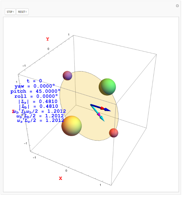

Root Finding

To step from

k-1

and

k+1

, find the root

k+1

(

k+1

(

k-1

, where

∈

⋆



(3)

is the integral of the virtual work of the external force over time interval

Start with a certain orientation and angular velocity:

In[]:=

o3={0,0,0};

In[]:=

(T0$=TSE3[initQuat$,o3])//SE3Form

Out[]//DisplayForm=

0.707107	0.	0.707107	0
0.	1.	0.	0
-0.707107	0.	0.707107	0
0	0	0	1

In[]:=

ClearAll[stepDzhanyRK4];With[{apparatus=dzhanybekhov},With[{ibibi=apparatus["moment of inertia"]},With[{Ib=ibibi〚1〛,Ibi=ibibi〚2〛},

stepDzhanyRK4

[Tk_,ωbIn_,h_,τs_:o3]:=Module[{ωb=ωbIn,rotMatSO3=pickSO3[Tk],ωs,Lb,Ls},{ωb,rotMatSO3,ωs,Lb,Ls}=oneStepSO3ForcedRotationalMotion[ωb,rotMatSO3,Ib,Ibi,h,τs];<|"TSE3"TSE3[rotMatSO3,o3],"ωb"ωb,"Lb"Lb,"ωs"->ωs,"Ls"Ls|>]]]];

In[]:=

ClearAll[adHocStep];adHocStep[T_,w_,h_]:=(step$=stepDzhanyRK4[T,w,h];wb$=step$["ωb"];Tkp$=step$["TSE3"]);adHocStep[T0$,initωb$,0.01];(T1$=Tkp$)//SE3Form

Out[]//DisplayForm=

0.707109	0.0423303	0.705836	0
0.00009994	0.998201	-0.059964	0
-0.707105	0.0424716	0.705832	0
0	0	0	1

In[]:=

adHocStep[T1$,wb$,0.01];(T2$=Tkp$)//SE3Form

Out[]//DisplayForm=

0.707119	0.084508	0.702026	0
0.000199122	0.992809	-0.119712	0
-0.707094	0.0847906	0.702017	0
0	0	0	1

DREPE should have magnitude close to zero.

In[]:=

DREPE[T0$,T1$,T2$,Gdzhany6R6,0&,0,

0.01

]//Norm

Out[]=

7.99789×

-9

T2$ is very nearly a root of DREPE. Is it close enough? Hard to say, yet, but we study the numerics below and we will refine the root with bandit search when needed (https://en.wikipedia.org/wiki/Multi-armed_bandit).

Adapt the step-by-step demonstration above to DREPE. The first step produces a macroscopic value of DREPE, that is, a failure to find a root. This failure is due only to the fact that DREPE requires two configuration estimates to bootstrap — we’ve seen this before in DELE. From the second step onward, the roots proposed by RK4 produce only microscopic values of DREPE, showing that the proposed roots are good for Dzhanybekhov. We suspect that they will not be good for 4DISP.

In[]:=

ClearAll[showSO3ApparatusWithDREPE];showSO3ApparatusWithDREPE[t_,ωb_,Lb_,ωs_,Ls_,Ib_,rotMatSO3_,DREPENorm_,apparatus_]:=Module{placeZ=1,y,p,r},With{arrowDiameter=0.02,displaceZ=-0.15},{y,p,r}=yprFromRotMat[rotMatSO3];ShowGraphics3DText[myFont[Blue]["t = "<>ToString[NumberForm[t,{10,2}]]],{-1,-1,placeZ}],placeZ+=displaceZ;Text[myFont[Blue]["|

DREPE

| = "<>ToString[NumberForm[DREPENorm,{10,6},NumberFormat(Row[{#1,"e",If[#3==="","0 ",#3]}]&)]]],{-.999,-1,placeZ}],placeZ+=displaceZ;Text[myFont[Blue]["yaw = "<>ToString[NumberForm[y/°,{10,4}]]<>"°"],{-.999,-1,placeZ}],placeZ+=displaceZ;Text[myFont[Blue]["pitch = "<>ToString[NumberForm[p/°,{10,4}]]<>"°"],{-.999,-1,placeZ}],placeZ+=displaceZ;Text[myFont[Blue]["roll = "<>ToString[NumberForm[r/°,{10,4}]]<>"°"],{-.999,-1,placeZ}],placeZ+=displaceZ;Text[myFont[Blue]["|

| = "<>ToString[NumberForm[Sqrt[Ls.Ls],{10,4}]]],{-.975,-1,placeZ}],placeZ+=displaceZ;Text[myFont[Blue]["|

| = "<>ToString[NumberForm[Sqrt[Lb.Lb],{10,4}]]],{-.975,-1,placeZ}],placeZ+=displaceZ;TextmyFont[Blue]"



/2 = "<>ToStringNumberFormSqrt

ωb.Ib.ωb,{10,4},{-.95,-1,placeZ},placeZ+=displaceZ;TextmyFont[Blue]"



/2 = "<>ToStringNumberFormSqrt

ωb.Lb,{10,4},{-.95,-1,placeZ},placeZ+=displaceZ;TextmyFont[Blue]"



/2 = "<>ToStringNumberFormSqrt

ωs.Ls,{10,4},{-.95,-1,placeZ},Magenta,Arrow[Tube[{o,Ls},arrowDiameter]],Text[myFont[Black,12]["Inertial-Frame Ang Mom"],{-1.9,+0.2,1},BackgroundMagenta],Red,Arrow[Tube[{o,Lb},arrowDiameter]],Text[myFont[Black,12]["Body-Frame Ang Mom"],{-1.7,-0.1,1},BackgroundRed],Cyan,Arrow[Tube[{o,ωs/10},arrowDiameter*1.10]],Text[myFont[Black,12]["Inertial-Frame Ang Vel"],{-1.4,-0.4,1},BackgroundCyan],Blue,Arrow[Tube[{o,ωb/10},arrowDiameter*1.10]],Text[myFont[White,12]["Body-Frame Ang Vel"],{-1.3,-0.7,1},BackgroundBlue],White,GeometricTransformation[apparatus["graphics primitives"],rotMatSO3],AxesTrue,PlotRangeConstantArray[plotRg,3],AxesLabelmyFont[Red]/@{"X","Y","Z"},ImageSizeLarge;With[{apparatus=dzhanybekhov,h=0.01,ωbIn={6.,.01,0.0},rqIn=rq[π/4.0,{0,1,0}],τs={0,0,0}},With[{ibibi=apparatus["moment of inertia"]},With[{Ib=ibibi〚1〛,Ibi=ibibi〚2〛},DynamicModule[{ωb=ωbIn,rotMatSO3=rotMatFromQ[rqIn],ωs,Lb,Ls,t=0,Tkm,Tk,Tkp,DREPENorm},With[{init=Function[(*ofnoarguments*)Tkm=Tk=TSE3[rqIn,o3];{ωb,rotMatSO3,ωs,Lb,Ls}=initialConditionsSO3ForcedRotationalMotion[ωbIn,rotMatFromQ[rqIn],Ib,Ibi];t=0;Tkp=TSE3[rotMatSO3,o3];DREPENorm=Norm[

DREPE[Tkm,Tk,Tkp,Gdzhany6R6,0&,0,h]

];

showSO3ApparatusWithDREPE

[t,ωb,Lb,ωs,Ls,Ib,rotMatSO3,DREPENorm,apparatus]],step=Function[(*ofnoarguments*)Tkm=Tk;Tk=Tkp;{ωb,rotMatSO3,ωs,Lb,Ls}=oneStepSO3ForcedRotationalMotion[ωb,rotMatSO3,Ib,Ibi,h,τs];Tkp=TSE3[rotMatSO3,o3];(*stillaquatinthesim*)DREPENorm=

Norm

[

DREPE[Tkm,Tk,Tkp,Gdzhany6R6,0&,0,h]

];t+=h;

showSO3ApparatusWithDREPE

[t,ωb,Lb,ωs,Ls,Ib,rotMatSO3,DREPENorm,apparatus]]},DynamicModule[{dpy=init[]},Manipulate[dpy,Row[{Button[" STEP ! ",dpy=step[]],Button[" RESET ! ",dpy=init[]]}],SaveDefinitions->True]]]]]]]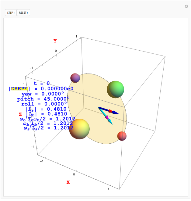

Adapt the continuous demonstration of Dzhanybekhov to CGDVIE3 and DREPE. This only tracks the microscopic values of DREPE; it does not update the roots, proposed by RK4. Note the time increment,

h=0.03

is three times larger (better) than we had with RK4. 0.03 is much too large to produce decent roots of DREPE for 4DISP; even

h=0.01

is too large for 4DISP.

In[]:=

ClearAll[runSimForcedRotationalMotionWithDREPE];runSimForcedRotationalMotionWithDREPE[apparatus_,h_,ωbIn_:{6.,.01,0},rqIn_:rq[π/4.0,{0,1.,0}],fs_:{0,0,0},τs_:{0,0,0}]:=With[{ibibi=apparatus["moment of inertia"]},With[{Ib=ibibi[[1]],Ibi=ibibi[[2]]},DynamicModule[{t=0,ωb=ωbIn,ωs,Lb,Ls,rotMatSO3=rotMatFromQ[rqIn],Tkm,Tk,Tkp,DREPENorm},With[{init=Function[(*ofnoarguments*)Tkm=Tk=TSE3[rqIn,o3];{ωb,rotMatSO3,ωs,Lb,Ls}=initialConditionsSO3ForcedRotationalMotion[ωbIn,rotMatFromQ[rqIn],Ib,Ibi];t=0;Tkp=TSE3[rotMatSO3,o3];DREPENorm=Norm[DREPE[Tkm,Tk,Tkp,Gdzhany6R6,0&,0,

]];showSO3ApparatusWithDREPE[t,ωb,Lb,ωs,Ls,Ib,rotMatSO3,DREPENorm,apparatus]],step=Function[(*ofnoarguments*)Tkm=Tk;Tk=Tkp;{ωb,rotMatSO3,ωs,Lb,Ls}=oneStepSO3ForcedRotationalMotion[ωb,rotMatSO3,Ib,Ibi,h,τs];Tkp=TSE3[rotMatSO3,o3];(*stillaquatinthesim*)DREPENorm=Norm[DREPE[Tkm,Tk,Tkp,Gdzhany6R6,0&,0,

]];t+=h;showSO3ApparatusWithDREPE[t,ωb,Lb,ωs,Ls,Ib,rotMatSO3,DREPENorm,apparatus]]},init[];Dynamic[t+=h;step[]]]]]];

This also loses energy and angular momentum, but more slowly than does TQDL & RK4 and at a time step 3 times more coarse — 0.3 instead of the .01 we needed with TDQL and RK4. This is a significant improvement. Note that the quantity |DREPE| is ideally zero. We see that it fluctuates around some small values, suggesting overall good performance.

In[]:=

runSimForcedRotationalMotionWithDREPE[dzhanybekhov,0.03]

Out[]=

We can’t do 4DISP yet because we don’t have a force model.

In[]:=

ClearAll[runSimForcedRotationalMotionWithDREPErig];runSimForcedRotationalMotionWithDREPErig[apparatus_,h_,ωbIn_:{6.,.01,0},rqIn_:rq[π/4.0,{0,1.,0}],fs_:{0,0,0},τs_:{0,0,0}]:=With[{ibibi=apparatus["moment of inertia"]},With[{Ib=ibibi[[1]],Ibi=ibibi[[2]]},DynamicModule[{t=0,ωb=ωbIn,ωs,Lb,Ls,rotMatSO3=rotMatFromQ[rqIn],Tkm,Tk,Tkp,DREPENorm,qk,csk,τsk,Fk},With[{init=Function[(*ofnoarguments*)Tkm=Tk=TSE3[rqIn,o3];{ωb,rotMatSO3,ωs,Lb,Ls}=initialConditionsSO3ForcedRotationalMotion[ωbIn,rotMatFromQ[rqIn],Ib,Ibi];t=0;Tkp=TSE3[rotMatSO3,o3];qk=qFromRotMat[rotMatSO3];csk=rv[qk,rig["cb"]];τsk=(rig["mass"]Abs[g]e3)csk;Fk=ConstantArray[-1.,6];DREPENorm=Norm[DREPE[Tkm,Tk,Tkp,Gdzhany6R6,PrigR,Fk,

]];t+=h;showSO3ApparatusWithDREPE[t,ωb,Lb,ωs,Ls,Ib,rotMatSO3,DREPENorm,apparatus]]},init[];Dynamic[t+=h;step[]]]]]];runSimForcedRotationalMotionWithDREPErig[rig,0.03,o,Q[0,10°,0*-0.5°],o]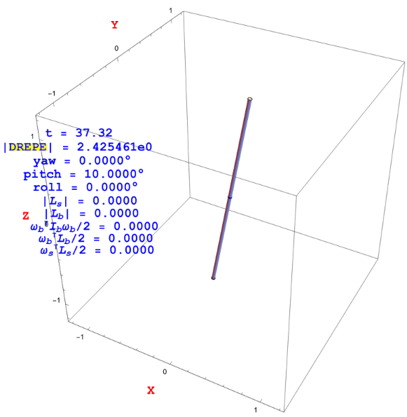

References

Jack B Kuipers, Quaternions and Rotation Sequences, Princeton University Press, 1999.

Jeongseok Lee, Karen Liu, Frank C. Park, Siddartha S. Srinivasa, A Linear-Time Variational Integrator for Multibody Systems, 2018, https://arxiv.org/abs/1609.02898

Ari Stern, Discrete Geometric Mechanics and Variational Integrators, 2006, http://ddg.cs.columbia.edu/SIGGRAPH06/stern-siggraph-talk.pdf.

Ethan Eade, Lie Groups for 2D and 3D Transformations, 2017, http://ethaneade.com/lie.pdf.

NIST: Digital Library of Mathematical Functions, https://dlmf.nist.gov.

Brian C. Hall, Lie Groups, Lie Algebras, and Representations, Second Edition, 2015, Springer.

Guangyu Liu, Modeling, stabilizing control and trajectory tracking of a spherical inverted pendulum, PhD thesis, 2007, University of Melbourne,
https://minerva-access.unimelb.edu.au/handle/11343/37225.

Wikipedia, Tennis-Racket Theorem, https://en.wikipedia.org/wiki/Tennis_racket_theorem.

Marin Kobilarov, Keenan Crane, Mathieu Desbrun, Lie Group Integrators for Animation and Control of Vehicles, 2009 (?).

Ari Stern, Mathieu Desbrun, Discrete Geometric Mechanics for Variational Time Integrators, 2006 (http://www.geometry.caltech.edu/pubs/SD06.pdf).

Kenth Engø, On The BCH Formula in (3), https://www.researchgate.net/profile/Kenth-Engo-Monsen/publication/233591614_On_the_BCH-formula_in_so3/links/004635199177f69467000000/On-the-BCH-formula-in-so3.pdf .

Alexander Van-Brunt, Max Visser, Explicit Baker-Campbell-Hausdorff formulae for some specific Lie algebras, https://arxiv.org/pdf/1505.04505.pdf.

Wikipedia, Baker-Campbell-Hausdorff Formula, https://en.wikipedia.org/wiki/Baker%E2%80%93Campbell%E2%80%93Hausdorff_formula.

Jerrold E. Marsden, Tudor S. Ratiu, Introduction to Mechanics and Symmetry, Second Edition, 2002

Moylan, Andrew, Stabilized Inverted Pendulum, https://blog.wolfram.com/2011/01/19/stabilized-inverted-pendulum/, and Stabilized n-Link Pendulum, https://blog.wolfram.com/2011/03/01/stabilized-n-link-pendulum/

Paul R. Halmos, Naive Set Theory, 2015.

David Lovelock and Hanno Rund, Tensors, Differential Forms, and Variational Principles, 1975.

Ralph Abraham and Jerrold E. Marsden, Foundations of Mechanics: 2nd Edition, 1980.

Taeyoung Lee, Melvin Leok, and N. Harris McClamroch, Discrete Control Systems, https://arxiv.org/abs/0705.3868.

Taeyoung Lee, Melvin Leok, N. Harris McClamroch, Global Formulations of Lagrangian and Hamiltonian Mechanics on Manifolds, Springer, https://a.co/d/0lTbL9t.

Tristan Needham, Visual Differential Geometry and Forms, https://a.co/d/9hoKekz.

xAct, Efficient tensor computer algebra for the Wolfram Language, http://xact.es/index.html.

Blanco, Jose-Luis, A tutorial on SE(3) transformation parameterizations and on-manifold optimization, Technical Report #012010, Universidad de Malaga (https://jinyongjeong.github.io/Download/SE3/jlblanco2010geometry3d_techrep.pdf).

Marsden and West has exhaustive treatment of Noether’s Theorem (http://www.cds.caltech.edu/~marsden/bib/2001/09-MaWe2001/MaWe2001.pdf).

Maxime Tournier, Notes on Lie Groups, https://maxime-tournier.github.io/notes/lie-groups.html.

John Baez, Javier P. Muniain, Gauge Fields, Knots and Gravity, (https://a.co/d/jdRnOU0)

CITE THIS NOTEBOOK

Geometric Discrete Variational Dynamics -- Part 1: Free Bodies
by Brian Beckman
Wolfram Community, STAFF PICKS, January 14, 2024
https://community.wolfram.com/groups/-/m/t/3103170

Abstract

Prior Failures

The Future: Discretized Lagrangians on Lie Groups

Tiny Quaternionic Dynamics Library (TQDL)

Primitives

Q: Quaternion From ψ, θ, ϕ

Forced Motion for TQDL & RK4

Demos of TQDL & RK4

Dzhanybekhov

Apparatus

Free Motion Demo (TQDL & RK4)

Forced Motion Demos (TQDL & RK4)

aCyl (apparatus)

Rod1 (apparatus)

Spherical Pendulum

ISSUE: Accumulating Energy and Angular Momentum

Addressing the Mystery

Demonstration of the Coordinate System

Dynamical Set-Up

Ground-Truth Solution with Initial Conditions

Plot the Solutions

Phase Portrait

Ground-Truth Animation

Discrete Lagrangian

Discrete Euler-Lagrange Equations

Visual Sanity Check

Numerical Solution for δ1 and η1

bootIntegrator

Utilities

Proofs and Tests

Conceptual Checks

Investigate Formulae

DREPE, DRNEA, and CGDVIE3 Theory

DRNEA (Reference 2)

SO(3), (3)

Definitions

Example

Naming Convention (Hungarian Types)

Vectors as Lists, Column Vectors, Row Vectors

hatSo3: 3(3), unHatR3: (3)3

expSO3: (3)SO(3), AKA Rodrigues’ Formula

logSo3: SO(3)(3)

Remarks

Adjoint in SO(3)

SE(3)

Definitions

SE3Form

pickSO3: SE(3)SO(3)

pickR3: SE(3)3

(3)

se3Form

hatSe3: 6(3), unHatR6: (3)6, unHat2R3: (3)2×3

expSE3: (3)SE(3)

logSe3: SE(3)(3), logR6: SE(3)6

ad6R6: (3)(3)6, Lie Bracket Operator

dlog6R6: (3)(3)6, Inverse Right Trivialized Tangent Operator

Adj6R6: Adjoint Operator in SE(3)

Lagrangian

TSE3: Configuration

VR6, VhatSe3: Velocity in (3)

PR, PrigR: Potential Energy

G6R6: Grig6R6: Inertial Matrix

LR, LrigR: Lagrangian

LdRigR: Trapezoidal Quadrature

Variational Integrators in SE(3) (TODO)

Root Finding

References

CITE THIS NOTEBOOK

Prior Failures


Forced Motion for TQDL & RK4


Spherical Pendulum


Dynamical Set-Up


Numerical Solution for
δ
1
and
η
1

Utilities


DREPE, DRNEA, and CGDVIE3 Theory


hatSo3:
3

(3)
, unHatR3:
(3)
3


expSO3:
(3)SO(3)
, AKA Rodrigues’ Formula

logSo3:
SO(3)(3)

pickSO3:
SE(3)SO(3)

pickR3:
SE(3)
3


hatSe3:
6

(3)
, unHatR6:
(3)
6

, unHat2R3:
(3)
2×3


expSE3:
(3)SE(3)

logSe3:
SE(3)(3)
, logR6:
SE(3)
6


ad6R6:
(3)(3)
6

, Lie Bracket Operator

dlog6R6:
(3)(3)
6

, Inverse Right Trivialized Tangent Operator

Variational Integrators in
SE(3)
(TODO)