Abstract
Abstract
Automatic labeling in visualization
◼
Where is automatic labeling used?
◼
Why automation?
◼
What is automated?
◼
How is it automated?
◼
When was it rolled out?
Where is labeling used?
Where is labeling used?
Applications of automatic labeling
Applications of automatic labeling
◼
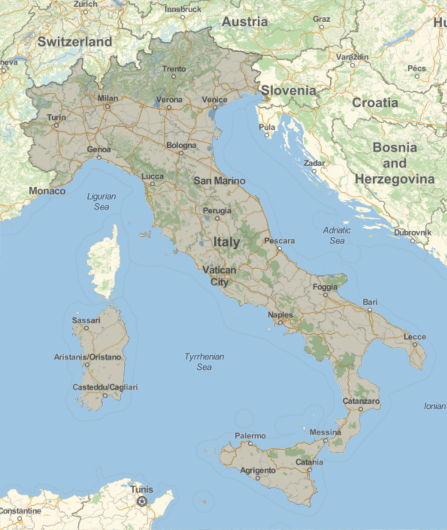
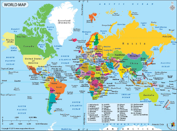
Map
GeoGraphics
◼
Data Analysis
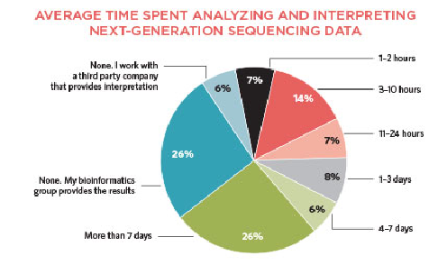
◼
Scientific Plots
◼
Anatomy
Why Automation?
Why Automation?
◼
Free-hand labeling can be time consuming and hard to reproduce.
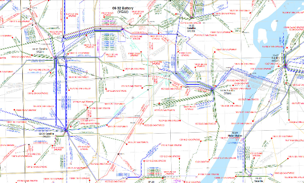
◼
Without an algorithmic method, labels can collide with each other and become hard to read.
◼
Using low level Text to add labels requires post-processing of the plots.
◼
Free-hand labeling can distract from the process of data exploration.
What is automated?
What is automated?
Data
Data
◼
Categorical data
◼
Meta data
Options
Options
◼
PlotLabels
◼
LabelingFunction
◼
PlotHighlighting
◼
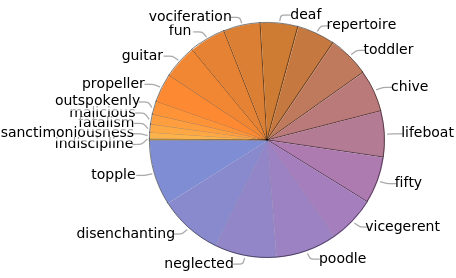
ChartLabels
Wrapper
Wrapper
◼
Callout
◼
Labeled
◼
Highlighted
Categorical data
Categorical data
◼
DateListStepPlot
◼
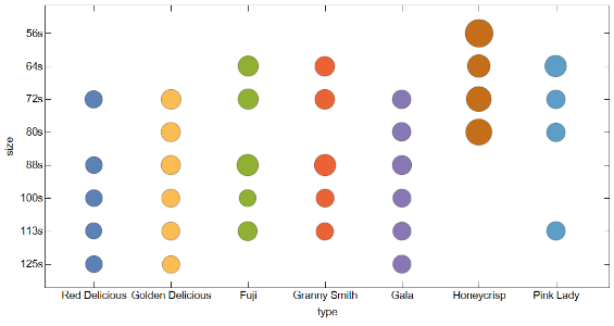
BubbleChart
In[]:=
Out[]=
{{{Red Delicious,72s,36.},{Red Delicious,88s,34.5},{Red Delicious,100s,34.5},{Red Delicious,113s,32.5},{Red Delicious,125s,34.5}},{{Golden Delicious,72s,46.5},{Golden Delicious,80s,45.},{Golden Delicious,88s,43.5},{Golden Delicious,100s,39.5},{Golden Delicious,113s,38.5},{Golden Delicious,125s,35.5}},{{Fuji,64s,48.5},{Fuji,72s,48.},{Fuji,88s,56.},{Fuji,100s,34.5},{Fuji,113s,44.}},{{Granny Smith,64s,46.5},{Granny Smith,72s,46.5},{Granny Smith,88s,54.},{Granny Smith,100s,38.5},{Granny Smith,113s,36.5}},{{Gala,72s,42.},{Gala,80s,42.},{Gala,88s,44.},{Gala,100s,39.5},{Gala,113s,39.},{Gala,125s,38.5}},{{Honeycrisp,56s,92.5},{Honeycrisp,64s,62.5},{Honeycrisp,72s,75.5},{Honeycrisp,80s,80.}},{{Pink Lady,64s,56.},{Pink Lady,72s,42.},{Pink Lady,80s,41.5},{Pink Lady,113s,42.}}}
In[]:=
BubbleChart,ScalingFunctions->{NominalScale[Automatic],NominalScale[{"125s","113s","100s","88s","80s","72s","64s","56s"}],None},AspectRatio12,FrameLabel->{{"size",None},{"type",None}},ImageSize->600
◼
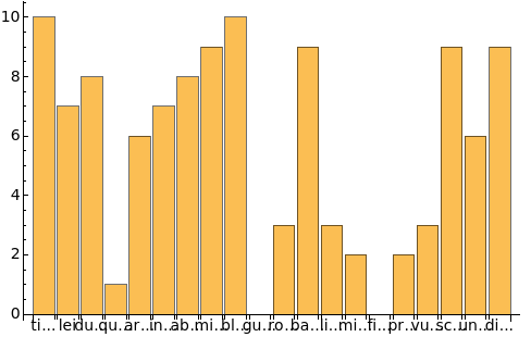
BarChart
◼
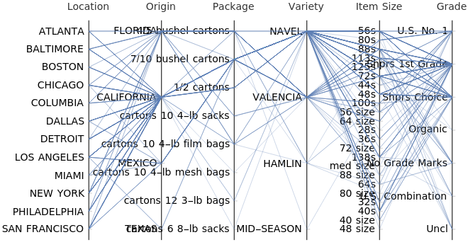
ParallelAxisPlot
In[]:=
Out[]//Short=
{{ATLANTA,FLORIDA,4/5 bushel cartons,NAVEL,56s,U.S. No. 1},236,{SAN FRANCISCO,MEXICO,7/10 bushel cartons,VALENCIA,113s,No Grade Marks}}
In[]:=
ParallelAxisPlot,ScalingFunctionsNominalScale[Automatic],AxesLabel->{"Location","Origin","Package","Variety","Item Size","Grade"},ImageSize1000,LabelStyle14
Out[]=
Highlighting labels
Highlighting labels
Line Labeling
Line Labeling
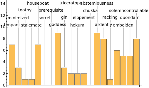
1D Point Labeling
1D Point Labeling
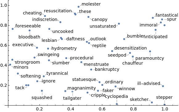
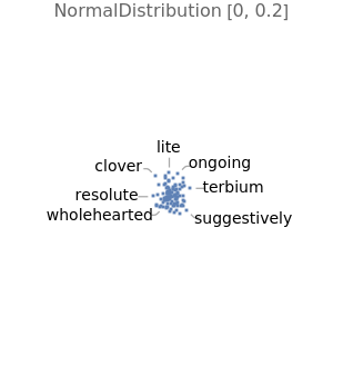
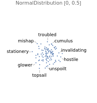
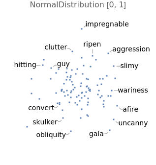
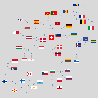
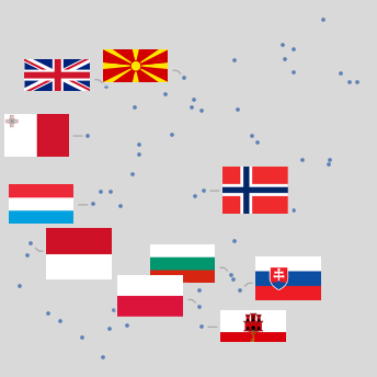
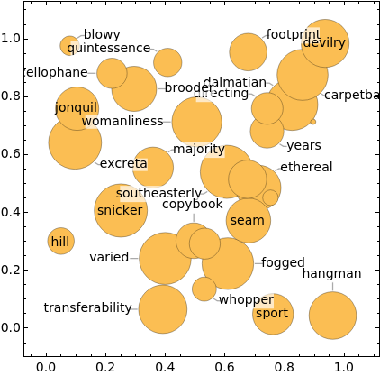
2D and 3D Point Labeling
2D and 3D Point Labeling
ListPlot[RandomReal[1,{50,2}]RandomWord[50]]
Out[]=
TableListPlotRandomVariate[NormalDistribution[0,σ],{100,2}]->RandomWord[100],,{σ,{0.2,0.5,1}}
Out[]=
,
,
In[]:=
FeatureSpacePlotEntityValue,"FlagImage",LabelingFunctionCallout

Out[]=
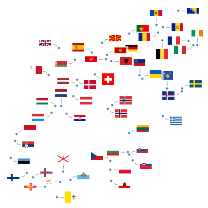
In[]:=
TableFeatureSpacePlotEntityValue,"FlagImage",LabelingFunctionCallout,LabelingSizesize,ImageSize360,BackgroundLightGray,{size,{20,60}}
Out[]=
,
Out[]=

Out[]=
 ,
, ,
,
Parametric Curve Labeling
Parametric Curve Labeling
Region Labeling
Region Labeling
Surface Labeling
Surface Labeling
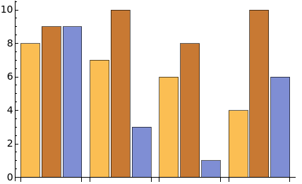
Labeling In Charts
Labeling In Charts
Out[]=
Out[]=
Out[]=
In[]:=
TableBarChart{1,1,2,3,5,8,13},ChartLabels->
,
,
,
,
,
,
,ImageSizesize,LabelingSizeAutomatic,BaselinePosition->Axis,{size,{200,400}}
Out[]=
Out[]=
How?
How?
Methods of implementation of automatic labeling
Image Processing
Image Processing
Optimization
Optimization
Geometry
Geometry
Point Feature Labeling Problem
Point Feature Labeling Problem
Others
Others
When is it rolled out?
When is it rolled out?
◼
Timeline of labeling
In[]:=
TimelinePlot[data,ImageSize1100,PlotRangePadding{{Scaled[0.1],Scaled[0.1]},None},AspectRatio1/1.75,PlotStyleColorData[108]]
Out[]=
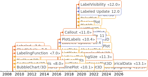
data
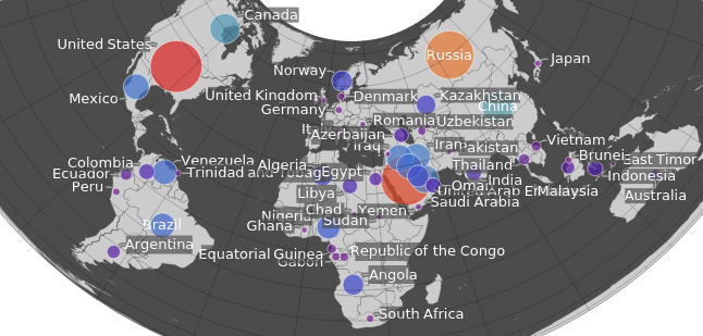
Showcases
Showcases
In[]:=
l=["Position"];c=["Name"];oil=;major=Quantile[QuantityMagnitude@DeleteMissing[oil],0.75];oildata=Select[Select[Transpose[{l,oil,c}],Head@#[[2]]=!=Missing&],QuantityMagnitude[#[[2]]]>major&];GeoBubbleChart[oildata[[All,1;;2]],ColorFunction"Rainbow",LabelingFunction(Callout[oildata[[All,3]][[#2[[2]]]],LabelStyle13]&),ImageSize1200,PlotTheme->"Marketing",GeoProjection"Albers"]
Out[]=
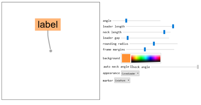
Callout Appearance
Callout Appearance
(*markup*)Callout[data,"label",LabelStyle40,LeaderSize{{leaderlength,angle,gap},{necklength,angle}},Appearanceappearance,CalloutMarkermarker,Backgroundbackgroundstyle,FrameMarginsframemargins,RoundingRadiusradius,CalloutStyleThickness[0.01]]
init
CITE THIS NOTEBOOK
CITE THIS NOTEBOOK
Wolfram R&D LIVE: Labeling Everywhere
by MinHsuan Peng
Wolfram Community, STAFF PICKS, September 6, 2023
https://community.wolfram.com/groups/-/m/t/3007543
by MinHsuan Peng
Wolfram Community, STAFF PICKS, September 6, 2023
https://community.wolfram.com/groups/-/m/t/3007543