CITE THIS NOTEBOOK: Working through exercises in Donald Knuth's Art of Computer Programming by Peter Burbery. Wolfram Community NOV 13 2022.
I decided to work through some exercises in Donald Knuth’s Art of Computer Programming Volume 4A Combinatorial Algorithms Part 1.
https://www.amazon.com/Computer-Programming-Volumes-1-4A-Boxed/dp/0321751043
https://www.amazon.com/Computer-Programming-Volumes-1-4A-Boxed/dp/0321751043
Exercise 41
Exercise 41
For what integers n do we have =? =?
K
n
P
n
K
n
C
n
In[]:=
Table[CompleteGraph[i],{i,9}]
Out[]=
,
,

,
,
,

,

,

,

In[]:=
Table[PathGraph[Range[i]],{i,9}]
Out[]=
,

,

,

,

,

,

,

,


I’ll use the new isomorphism functionality introduced in recent releases of Mathematica:
In[]:=
FindGraphIsomorphism
,
Out[]=
{11}
In[]:=
Names["*Isom*"]
Out[]=
{FindGraphIsomorphism,FindIsomers,FindIsomorphicSubgraph,FindSubgraphIsomorphism,IsomorphicGraphQ,IsomorphicSubgraphQ}
In[]:=
Information/@Names["*Isom*"]
Out[]=
,,,,,
In[]:=
Select[IsomorphicGraphQ[CompleteGraph[#],PathGraph[Range[#]]]&][Range[10]]
Out[]=
{1,2}
In[]:=
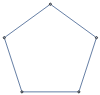
Select[IsomorphicGraphQ[CompleteGraph[#],CycleGraph[#]]&][Range[10]]
Out[]=
{3}
Donald Knuth lists 0 as an answer as well in addition to 3, but I don’t think the 0 graph exists or makes sense.
Exercise 43
Exercise 43
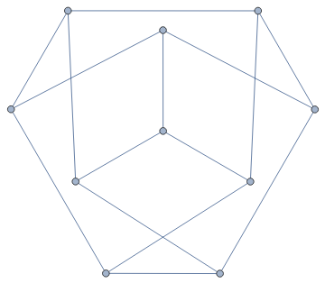
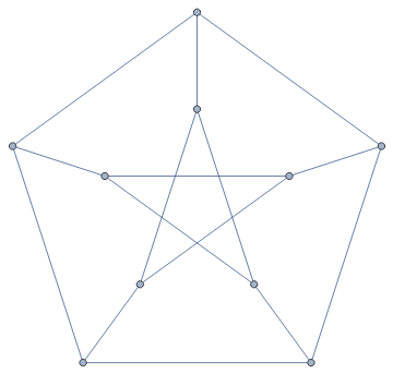
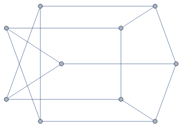
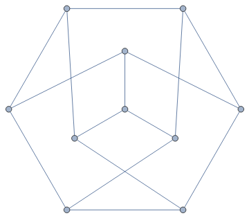
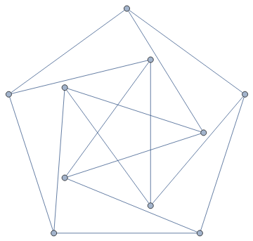
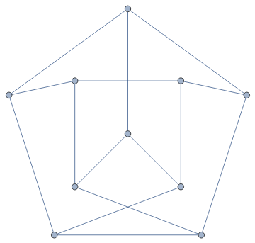
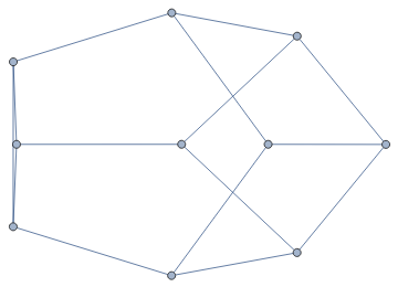
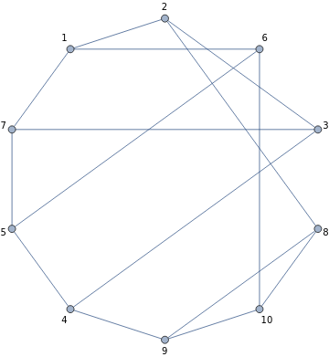
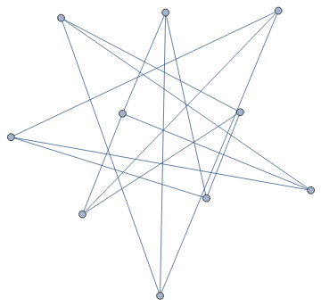
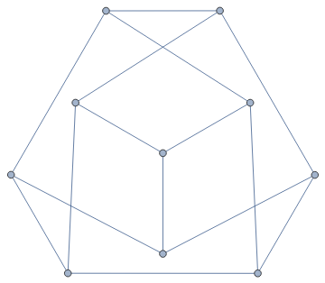
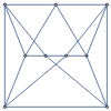
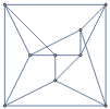
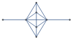
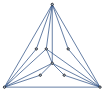
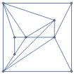
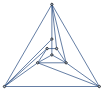
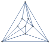
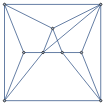
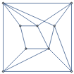
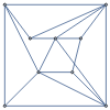
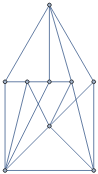
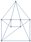
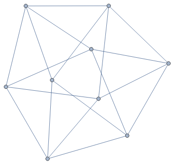
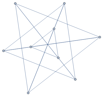
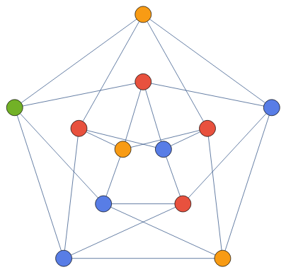
Are any of the following graphs the same as the Petersen graph?
I have a hard copy edition of the Art of Computer Programming that I am using to answer this exercise.
In[]:=
GraphData["PetersenGraph"]
Out[]=

In[]:=
Graph[{1<->2,2<->3,3<->4,4<->5,5<->6,6<->7,7<->8,8<->9,1<->5,9<->1,2<->7,3<->10,9<->10,6<->10,4<->8}]
Out[]=
In[]:=
IsomorphicGraphQ[Graph[{1<->2,2<->3,3<->4,4<->5,5<->6,6<->7,7<->8,8<->9,1<->5,9<->1,2<->7,3<->10,9<->10,6<->10,4<->8}],GraphData["PetersenGraph"]]
Out[]=
True
In[]:=
FindGraphIsomorphism[Graph[{1<->2,2<->3,3<->4,4<->5,5<->6,6<->7,7<->8,8<->9,1<->5,9<->1,2<->7,3<->10,9<->10,6<->10,4<->8}],GraphData["PetersenGraph"]]
Out[]=
{11,24,32,45,53,68,79,810,96,107}
In[]:=
GraphData["PetersenGraph","Embeddings"]
Out[]=
{{0.,1.},{-0.951,0.309},{-0.588,-0.809},{0.588,-0.809},{0.951,0.309},{0.,2.},{-1.902,0.618},{-1.176,-1.618},{1.176,-1.618},{1.902,0.618}},{{0.323,0.975},{0.037,0.789},{0.037,0.186},{0.323,0.},{0.5,0.487},{1.287,0.975},{1.,0.789},{1.,0.186},{1.287,0.},{1.464,0.487}},{{0.448354,-0.269958},{0.60481,-0.338987},{0.586329,-0.50903},{0.586329,-0.0309114},{0.862447,-0.50903},{0.724304,-0.131983},{0.724304,-0.269958},{0.843797,-0.338987},{0.862447,-0.0309114},{1.,-0.269958}},{{0.448354,-0.269958},{0.606498,-0.145654},{0.529114,-0.0747932},{0.529114,-0.465148},{0.84211,-0.145654},{1.,-0.269958},{0.919831,-0.0747932},{0.724304,0.00606582},{0.724304,-0.545992},{0.919831,-0.465148}},{{0.454407,-0.222966},{0.632542,-0.53161},{0.549237,-0.0587373},{0.487373,-0.409661},{0.822119,-0.53161},{1.,-0.222966},{0.905932,-0.0587373},{0.727373,0.00609153},{0.727373,-0.271102},{0.967797,-0.409661}},{{0.602252,-0.541848},{0.734705,-0.312345},{0.668478,-0.656599},{0.668478,-0.427096},{0.867236,-0.312345},{1.,-0.541848},{0.93323,-0.656599},{0.801242,-0.656599},{0.801242,-0.503571},{0.93323,-0.427096}},{{0,0},{1,3},{0,4},{1,1},{4,4},{2,0},{2,2},{3,3},{3,1},{4,0}},{{2,2},{6,4},{4,2},{2,4},{6,2},{5,5},{6,6},{4,6},{2,6},{3,5}},,0,,-(5+,(-1+(5+,(1-,0,(5+,(-1-(5-,-,-,-(1+(5-,{{0.535302,0.95889},{0.328164,0.677274},{0.535302,0.470135},{0.0706049,0.621205},{0.328164,0.262996},{1.,0.621205},{0.742441,0.677274},{0.742441,0.262996},{0.247912,0.0745965},{0.822693,0.0745965}},-,(-1-(5-,(-1-+,(-1+(5-,(-1-(5+,(-1+(5+,(-1+(5+,(-1+(5-,(-1-
2
5+
5
1
2
1-
,2
5
1
2
1
2
1
10
5
)1
4
5
),-1
2
1
10
5
)1
4
5
),1
2
1-
,-2
5
1
2
1
10
5
)1
4
5
),1
2
1
10
5
)1
2
1
2
1+
,2
5
1
2
1
2
1+
,2
5
1
4
5
),1
2
1
10
5
)5
8
5
8
1
4
5
),{0,1},1
2
5
)1
2
5
),5
8
5
8
1
4
5
),{0,2},-1
2
1
2
5
)1
4
5
),-1
2
1
2
5
)1
4
5
),-1
2
5
)1
2
5
),1
2
5
)1
2
5
),-1
2
5
)1
2
5
)In[]:=
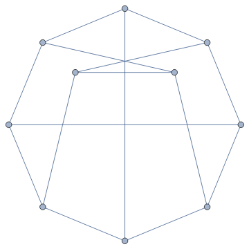
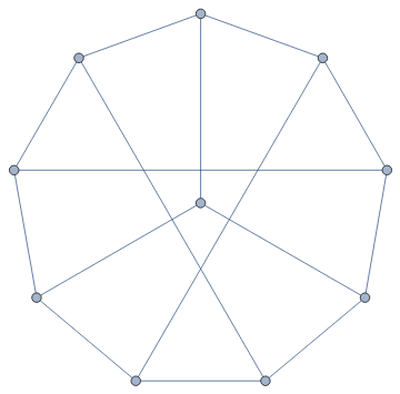
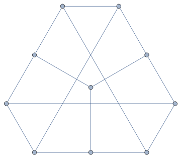
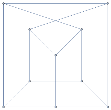
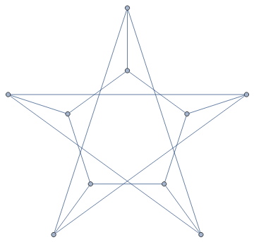
Length[GraphData["PetersenGraph","Embeddings"]]
Out[]=
11
In[]:=
Graph[GraphData["PetersenGraph"],VertexCoordinates->#]&/@GraphData["PetersenGraph","Embeddings"]
Out[]=
,
,
,
,
,
,
,
,
,
,
In[]:=
Graph[{1<->2,2<->3,3<->4,4<->5,5<->6,6<->1,1<->7,3<->7,5<->7,2<->8,4<->9,6<->10,8<->9,9<->10,8<->10}]
Out[]=
In[]:=
Graph[{1<->2,2<->3,3<->4,4<->5,5<->6,6<->1,1<->7,3<->7,5<->7,2<->8,4<->9,6<->10,8<->9,9<->10,8<->10},GraphLayout->"CircularEmbedding",VertexLabels->Automatic]
Out[]=
In[]:=
IsomorphicGraphQ[Graph[{1<->2,2<->3,3<->4,4<->5,5<->6,6<->1,1<->7,3<->7,5<->7,2<->8,4<->9,6<->10,8<->9,9<->10,8<->10},GraphLayout->"CircularEmbedding",VertexLabels->Automatic],GraphData["PetersenGraph"]]
Out[]=
False
In[]:=
FindGraphIsomorphismGraphData["PetersenGraph"],
Out[]=
{11,22,33,44,55,66,77,88,99,1010}
FindGraphIsomorphismGraphData["PetersenGraph"],
In[]:=
FindGraphIsomorphismGraphData["PetersenGraph"],
Out[]=
{11,22,33,44,55,66,77,88,99,1010}
In[]:=
FindGraphIsomorphism
,GraphData["PetersenGraph"]
Out[]=
{11,22,33,44,55,66,77,88,99,1010}
Exercise 44
Exercise 44
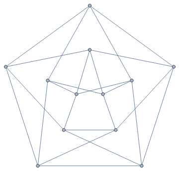
How many symmetries does Chvàtal’s graph have?
In[]:=
GraphData["ChvatalGraph"]
Out[]=
In[]:=
GraphData["ChvatalGraph","AutomorphismCount"]
Out[]=
8
There are 8 symmetries.
Exercise 45
Exercise 45
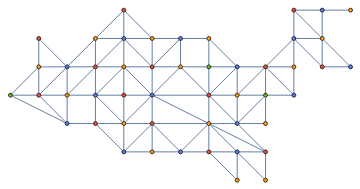
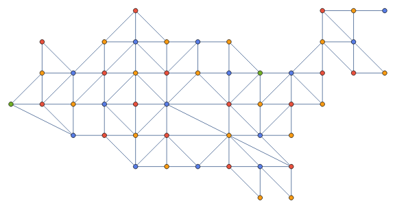
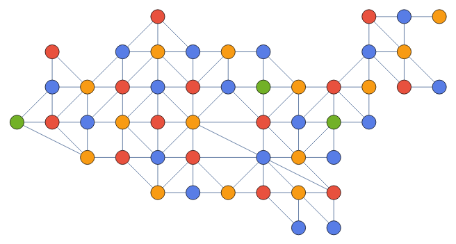
Find an easy way to 4-color the planar graph (17). Would 3 colors suffice?
In[]:=
GraphData["ContiguousUSAGraph"]
Out[]=

In[]:=
VertexCount[GraphData["ContiguousUSAGraph"]]
Out[]=
49
In[]:=
GraphData["ContiguousUSAGraph","ChromaticNumber"]
Out[]=
4
The minimum number of colors possible is 4.
In[]:=
FindVertexColoring[GraphData["ContiguousUSAGraph"]]
Out[]=
{3,1,2,2,1,3,1,2,1,2,2,4,3,3,1,1,2,3,1,3,3,2,1,1,1,3,2,1,3,2,3,1,3,1,1,2,2,2,1,3,2,3,1,4,1,1,3,2,3}
I can use a resource function I created to color a graph:
In[]:=
ResourceSearch["*color*graph*"]
Out[]=
In[]:=
PersistResourceFunction[{"ColorGraphVertices"}]
Out[]=
Success
In[]:=
ColorGraphVertices[GraphData["ContiguousUSAGraph"]]
Out[]=
In[]:=
ColorGraphVertices[GraphData["ContiguousUSAGraph"],ImageSize->Large]
Out[]=
In[]:=
ColorGraphVertices[GraphData["ContiguousUSAGraph"],ImageSize->Full,VertexSize->Large]
Out[]=
Exercise 46
Exercise 46
Let G with a graph with vertices, defined by a planar diagram that is “maximal,” in the sense that no additional lines can be drawn between nonadjacent vertices without crossing an existing edge.
n>=3
The graph data property I am looking for is “Triangulated” or “maximally planar”.
In[]:=
GraphData["Triangulated"]
Out[]=
{{Apollonian,2},{Apollonian,3},{Apollonian,4},{Apollonian,5},{Apollonian,6},{ChromaticallyEquivalent,{11,1,1}},{ChromaticallyEquivalent,{11,1,2}},{ChromaticallyEquivalent,{11,2,1}},{ChromaticallyEquivalent,{11,2,2}},{ChromaticallyEquivalent,{11,3,1}},{ChromaticallyEquivalent,{11,3,2}},{ChromaticallyEquivalent,{12,1,1}},{ChromaticallyEquivalent,{12,1,2}},{ChromaticallyEquivalent,{13,1,1}},{ChromaticallyEquivalent,{13,1,2}},{ChromaticallyEquivalent,{13,1,3}},{ChromaticallyEquivalent,{13,2,1}},{ChromaticallyEquivalent,{13,2,2}},{ChromaticallyEquivalent,{14,1,1}},{ChromaticallyEquivalent,{14,1,2}},{ChromaticallyEquivalent,{14,2,1}},{ChromaticallyEquivalent,{14,2,2}},{ChromaticallyEquivalent,{14,3,1}},{ChromaticallyEquivalent,{14,3,2}},{ChromaticallyEquivalent,{14,4,1}},{ChromaticallyEquivalent,{14,4,2}},{ChromaticallyEquivalent,{15,1,1}},{ChromaticallyEquivalent,{15,1,2}},{ChromaticallyEquivalent,{15,1,3}},{ChromaticallyEquivalent,{15,2,1}},{ChromaticallyEquivalent,{15,2,2}},{ChromaticallyEquivalent,{15,3,1}},{ChromaticallyEquivalent,{15,3,2}},{ChromaticallyEquivalent,{15,4,1}},{ChromaticallyEquivalent,{15,4,2}},{ChromaticallyEquivalent,{15,5,1}},{ChromaticallyEquivalent,{15,5,2}},{ChromaticallyEquivalent,{15,6,1}},{ChromaticallyEquivalent,{15,6,2}},{ChromaticallyEquivalent,{16,1,1}},{ChromaticallyEquivalent,{16,1,2}},{ChromaticallyEquivalent,{16,2,1}},{ChromaticallyEquivalent,{16,2,2}},{ChromaticallyEquivalent,{16,3,1}},{ChromaticallyEquivalent,{16,3,2}},{ChromaticallyEquivalent,{16,4,1}},{ChromaticallyEquivalent,{16,4,2}},{ChromaticallyEquivalent,{16,5,1}},{ChromaticallyEquivalent,{16,5,2}},{ChromaticallyEquivalent,{16,6,1}},{ChromaticallyEquivalent,{16,6,2}},{ChromaticallyEquivalent,{16,7,1}},{ChromaticallyEquivalent,{16,7,2}},{ChromaticallyEquivalent,{16,8,1}},{ChromaticallyEquivalent,{16,8,2}},{ChromaticallyEquivalent,{16,9,1}},{ChromaticallyEquivalent,{16,9,2}},{ChromaticallyEquivalent,{17,1,1}},{ChromaticallyEquivalent,{17,1,2}},{Dipyramid,3},{Dipyramid,5},{Dipyramid,6},{Dipyramid,7},{Dipyramid,8},{Dipyramid,9},{Dipyramid,10},{Dipyramid,11},{Dipyramid,12},{Dipyramid,13},{Dipyramid,14},{Dipyramid,15},{Dipyramid,16},{Dipyramid,17},{Dipyramid,18},{Dipyramid,19},{Dipyramid,20},DisdyakisDodecahedralGraph,DisdyakisTriacontahedralGraph,ErreraGraph,FritschGraph,GoldnerHararyGraph,HeawoodFourColorGraph,{Heptahedral,15},{Heptahedral,29},{Heptahedral,34},{Hexahedral,5},IcosahedralGraph,{JohnsonSkeleton,17},{JohnsonSkeleton,84},KittellGraph,McGregorGraph,MooreGraph,OctahedralGraph,PentakisDodecahedralGraph,PentakisIcosidodecahedralGraph,PoussinGraph,{SierpinskiTetrahedron,2},SmallTriakisOctahedralGraph,TetrahedralGraph,TetrakisHexahedralGraph,TriakisIcosahedralGraph,TriakisTetrahedralGraph,TriangleGraph,{Triangulated,{8,2}},{Triangulated,{8,3}},{Triangulated,{8,4}},{Triangulated,{8,5}},{Triangulated,{8,6}},{Triangulated,{8,8}},{Triangulated,{8,9}},{Triangulated,{8,10}},{Triangulated,{8,11}},{Triangulated,{8,12}},{Triangulated,{8,14}}}
Prove that the diagram partitions the plane into regions that each have exactly three vertices on their boundary. (One of these regions is the set of all points that lie outside the diagram.)
Therefore G has exactly 3n-6 edges.
I think there’s a graph function that does something with a plane.
In[]:=
Names["*plan*",IgnoreCase->True]
Out[]=
{ClipPlanes,ClipPlanesStyle,CoplanarPoints,DualPlanarGraph,ExoplanetData,FindPlanarColoring,HalfPlane,Hyperplane,InfinitePlane,MinorPlanetData,PlanarAngle,PlanarFaceList,PlanarGraph,PlanarGraphQ,PlanckRadiationLaw,PlaneCurveData,PlanetaryMoonData,PlanetData,PlantData,PlotRangeClipPlanesStyle}
In[]:=
Information/@Names["*plan*",IgnoreCase->True]
,,,,
Select graphs with at least three vertices:
I was running this in 13.2 but I got an error so I had to evaluate it in 13.1.
This is the error in 13.2
In[]:=
$Version
Out[]=
13.2.0 for Microsoft Windows (64-bit) (November 6, 2022)
In[]:=
triangulatedGraphsWithAtLastThreeVertices=Select[VertexCount[GraphData[#]]>=3&][GraphData["Triangulated"]]

Out[]=
{{Apollonian,2},{Apollonian,3},{Apollonian,4},{Apollonian,5},{Apollonian,6},{ChromaticallyEquivalent,{11,1,1}},{ChromaticallyEquivalent,{11,1,2}},{ChromaticallyEquivalent,{11,2,1}},{ChromaticallyEquivalent,{11,2,2}},{ChromaticallyEquivalent,{11,3,1}},{ChromaticallyEquivalent,{11,3,2}},{ChromaticallyEquivalent,{12,1,1}},{ChromaticallyEquivalent,{12,1,2}},{ChromaticallyEquivalent,{13,1,1}},{ChromaticallyEquivalent,{13,1,2}},{ChromaticallyEquivalent,{13,1,3}},{ChromaticallyEquivalent,{13,2,1}},{ChromaticallyEquivalent,{13,2,2}},{ChromaticallyEquivalent,{14,1,1}},{ChromaticallyEquivalent,{14,1,2}},{ChromaticallyEquivalent,{14,2,1}},{ChromaticallyEquivalent,{14,2,2}},{ChromaticallyEquivalent,{14,3,1}},{ChromaticallyEquivalent,{14,3,2}},{ChromaticallyEquivalent,{14,4,1}},{ChromaticallyEquivalent,{14,4,2}},{ChromaticallyEquivalent,{15,1,1}},{ChromaticallyEquivalent,{15,1,2}},{ChromaticallyEquivalent,{15,1,3}},{ChromaticallyEquivalent,{15,2,1}},{ChromaticallyEquivalent,{15,2,2}},{ChromaticallyEquivalent,{15,3,1}},{ChromaticallyEquivalent,{15,3,2}},{ChromaticallyEquivalent,{15,4,1}},{ChromaticallyEquivalent,{15,4,2}},{ChromaticallyEquivalent,{15,5,1}},{ChromaticallyEquivalent,{15,5,2}},{ChromaticallyEquivalent,{15,6,1}},{ChromaticallyEquivalent,{15,6,2}},{ChromaticallyEquivalent,{16,1,1}},{ChromaticallyEquivalent,{16,1,2}},{ChromaticallyEquivalent,{16,2,1}},{ChromaticallyEquivalent,{16,2,2}},{ChromaticallyEquivalent,{16,3,1}},{ChromaticallyEquivalent,{16,3,2}},{ChromaticallyEquivalent,{16,4,1}},{ChromaticallyEquivalent,{16,4,2}},{ChromaticallyEquivalent,{16,5,1}},{ChromaticallyEquivalent,{16,5,2}},{ChromaticallyEquivalent,{16,6,1}},{ChromaticallyEquivalent,{16,6,2}},{ChromaticallyEquivalent,{16,7,1}},{ChromaticallyEquivalent,{16,7,2}},{ChromaticallyEquivalent,{16,8,1}},{ChromaticallyEquivalent,{16,8,2}},{ChromaticallyEquivalent,{16,9,1}},{ChromaticallyEquivalent,{16,9,2}},{ChromaticallyEquivalent,{17,1,1}},{ChromaticallyEquivalent,{17,1,2}},{Dipyramid,3},{Dipyramid,5},{Dipyramid,6},{Dipyramid,7},{Dipyramid,8},{Dipyramid,9},{Dipyramid,10},{Dipyramid,11},{Dipyramid,12},{Dipyramid,13},{Dipyramid,14},{Dipyramid,15},{Dipyramid,16},{Dipyramid,17},{Dipyramid,18},{Dipyramid,19},{Dipyramid,20},DisdyakisDodecahedralGraph,DisdyakisTriacontahedralGraph,ErreraGraph,FritschGraph,GoldnerHararyGraph,HeawoodFourColorGraph,{Heptahedral,15},{Heptahedral,29},{Heptahedral,34},{Hexahedral,5},IcosahedralGraph,{JohnsonSkeleton,17},{JohnsonSkeleton,84},KittellGraph,McGregorGraph,MooreGraph,OctahedralGraph,PentakisDodecahedralGraph,PentakisIcosidodecahedralGraph,PoussinGraph,{SierpinskiTetrahedron,2},SmallTriakisOctahedralGraph,TetrahedralGraph,TetrakisHexahedralGraph,TriakisIcosahedralGraph,TriakisTetrahedralGraph,{Triangulated,{8,2}},{Triangulated,{8,3}},{Triangulated,{8,4}},{Triangulated,{8,5}},{Triangulated,{8,6}},{Triangulated,{8,8}},{Triangulated,{8,9}},{Triangulated,{8,10}},{Triangulated,{8,11}},{Triangulated,{8,12}},{Triangulated,{8,14}}}
This is the evaluation in 13.1
In[]:=
$Version
Out[]=
13.1.0 for Microsoft Windows (64-bit) (June 16, 2022)
In[]:=
triangulatedGraphsWithAtLastThreeVertices=Select[VertexCount[GraphData[#]]>=3&][GraphData["Triangulated"]]
Out[]=
{{Apollonian,2},{Apollonian,3},{Apollonian,4},{Apollonian,5},{Apollonian,6},{ChromaticallyEquivalent,{11,1,1}},{ChromaticallyEquivalent,{11,1,2}},{ChromaticallyEquivalent,{11,2,1}},{ChromaticallyEquivalent,{11,2,2}},{ChromaticallyEquivalent,{11,3,1}},{ChromaticallyEquivalent,{11,3,2}},{ChromaticallyEquivalent,{12,1,1}},{ChromaticallyEquivalent,{12,1,2}},{ChromaticallyEquivalent,{13,1,1}},{ChromaticallyEquivalent,{13,1,2}},{ChromaticallyEquivalent,{13,1,3}},{ChromaticallyEquivalent,{13,2,1}},{ChromaticallyEquivalent,{13,2,2}},{ChromaticallyEquivalent,{14,1,1}},{ChromaticallyEquivalent,{14,1,2}},{ChromaticallyEquivalent,{14,2,1}},{ChromaticallyEquivalent,{14,2,2}},{ChromaticallyEquivalent,{14,3,1}},{ChromaticallyEquivalent,{14,3,2}},{ChromaticallyEquivalent,{14,4,1}},{ChromaticallyEquivalent,{14,4,2}},{ChromaticallyEquivalent,{15,1,1}},{ChromaticallyEquivalent,{15,1,2}},{ChromaticallyEquivalent,{15,1,3}},{ChromaticallyEquivalent,{15,2,1}},{ChromaticallyEquivalent,{15,2,2}},{ChromaticallyEquivalent,{15,3,1}},{ChromaticallyEquivalent,{15,3,2}},{ChromaticallyEquivalent,{15,4,1}},{ChromaticallyEquivalent,{15,4,2}},{ChromaticallyEquivalent,{15,5,1}},{ChromaticallyEquivalent,{15,5,2}},{ChromaticallyEquivalent,{15,6,1}},{ChromaticallyEquivalent,{15,6,2}},{ChromaticallyEquivalent,{16,1,1}},{ChromaticallyEquivalent,{16,1,2}},{ChromaticallyEquivalent,{16,2,1}},{ChromaticallyEquivalent,{16,2,2}},{ChromaticallyEquivalent,{16,3,1}},{ChromaticallyEquivalent,{16,3,2}},{ChromaticallyEquivalent,{16,4,1}},{ChromaticallyEquivalent,{16,4,2}},{ChromaticallyEquivalent,{16,5,1}},{ChromaticallyEquivalent,{16,5,2}},{ChromaticallyEquivalent,{16,6,1}},{ChromaticallyEquivalent,{16,6,2}},{ChromaticallyEquivalent,{16,7,1}},{ChromaticallyEquivalent,{16,7,2}},{ChromaticallyEquivalent,{16,8,1}},{ChromaticallyEquivalent,{16,8,2}},{ChromaticallyEquivalent,{16,9,1}},{ChromaticallyEquivalent,{16,9,2}},{ChromaticallyEquivalent,{17,1,1}},{ChromaticallyEquivalent,{17,1,2}},{Dipyramid,3},{Dipyramid,5},{Dipyramid,6},{Dipyramid,7},{Dipyramid,8},{Dipyramid,9},{Dipyramid,10},{Dipyramid,11},{Dipyramid,12},{Dipyramid,13},{Dipyramid,14},{Dipyramid,15},{Dipyramid,16},{Dipyramid,17},{Dipyramid,18},{Dipyramid,19},{Dipyramid,20},DisdyakisDodecahedralGraph,DisdyakisTriacontahedralGraph,ErreraGraph,FritschGraph,GoldnerHararyGraph,HeawoodFourColorGraph,{Heptahedral,15},{Heptahedral,29},{Heptahedral,34},{Hexahedral,5},IcosahedralGraph,{JohnsonSkeleton,17},{JohnsonSkeleton,84},KittellGraph,McGregorGraph,MooreGraph,OctahedralGraph,PentakisDodecahedralGraph,PoussinGraph,{SierpinskiTetrahedron,2},SmallTriakisOctahedralGraph,TetrahedralGraph,TetrakisHexahedralGraph,TriakisIcosahedralGraph,TriakisTetrahedralGraph,TriangleGraph,{Triangulated,{8,2}},{Triangulated,{8,3}},{Triangulated,{8,4}},{Triangulated,{8,5}},{Triangulated,{8,6}},{Triangulated,{8,8}},{Triangulated,{8,9}},{Triangulated,{8,10}},{Triangulated,{8,11}},{Triangulated,{8,12}},{Triangulated,{8,14}}}
In[]:=
PlanarFaceList[GraphData[#]]&/@triangulatedGraphsWithAtLastThreeVertices
Out[]=
I am going to work on creating a function to make a planar coloring. I used the code from ColorGraphEdges to build a new function ColorPlanarGraphFaces.
In[]:=
ResourceFunction["ResourceFunctionDefinitionViewer"]["ColorGraphEdges"]
Out[]=
NotebookObject

Here is an example:
In[]:=
ResourceFunction[CloudObject["https://www.wolframcloud.com/obj/burbery1/DeployedResources/Function/ColorPlanarGraphFaces"]][GraphData[{"ChromaticallyEquivalent",{16,6,1}}]]
Out[]=
I can compare the number of vertices n with the number of edges which should be 3n-6.
In[]:=
AllTrue[triangulatedGraphsWithAtLastThreeVertices,3VertexCount[GraphData[#]]-6==EdgeCount[GraphData[#]]&]
Out[]=
True
This is true for all graphs.
Exercise 47
Exercise 47
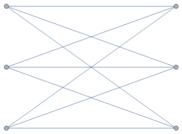
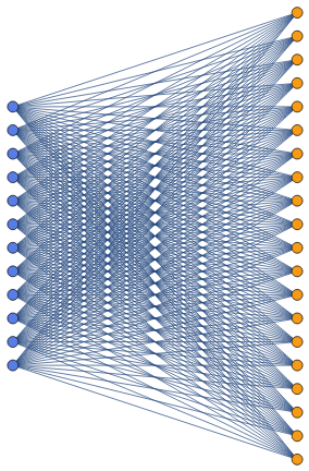
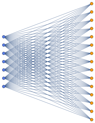
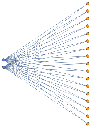
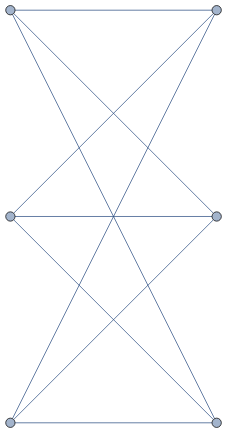
Prove that the complete bigraph isn’t planar.
K
3,3
This is related to the famous three utilities problem. It is well-known that you connect three houses to each other so each one has water, gas, and electricity. This means the complete bipartite graph is not planar and cannot be embedded in the plane. This graph can however, be embedded on a torus. The toroidal embedding of this graph could be used to create a solution to the three utilities on a torus or donut or coffee cup or tire or other object that topologically homeomorphic to a torus.
K
3,3
In[]:=
CompleteGraph[{3,3}]
Out[]=
In[]:=
PlanarGraphQ[CompleteGraph[{3,3}]]
Out[]=
False
Find the canonical graph:
In[]:=
CanonicalGraph[CompleteGraph[{3,3}]]
Out[]=
Find the name of the graph data entry:
In[]:=
GraphData[{"CompleteBipartite",{3,3}}]
Out[]=

Verify the graphs are isomorphic:
In[]:=
IsomorphicGraphQ[GraphData[{"CompleteBipartite",{3,3}}],CompleteGraph[{3,3}]]
Out[]=
True
In[]:=
GraphData[{"CompleteBipartite",{3,3}},"Planar"]
Out[]=
False
The property apices is the list of vertices whose removal renders the graph planar:
In[]:=
GraphData[{"CompleteBipartite",{3,3}},"Apices"]
Out[]=
{1,2,3,4,5,6}
Exercise 48
Exercise 48
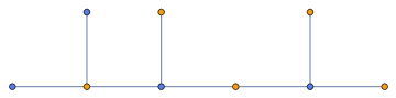
Complete the proof of Theorem B by showing that the stated procedure never the same color to two adjacent vertices.
Theorem B: A graph is bipartite if and only if it contains no cycle of odd length.
Conversely, if a graph contains no odd cycles we can color its vertices with the two colors {0,1} by carrying out the following procedure: Begin with all vertices uncolored. If all neighbors of colored vertices are already colored, choose an uncolored vertex , and color it 0. Otherwise choose a colored vertex that has an uncolored neighbor ; assign to the opposite color. Exercise 48 proves that a valid 2-coloring is eventually obtained.
w
u
v
v
I will use examples to demonstrate a case for this.
In[]:=
GraphData["Bipartite"]
Out[]=
I will verify that all bipartite graphs have a chromatic number of two.
In[]:=
AllTrue[GraphData["Bipartite"],GraphData[#,"ChromaticNumber"]==2&]
Out[]=
False
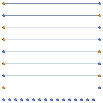
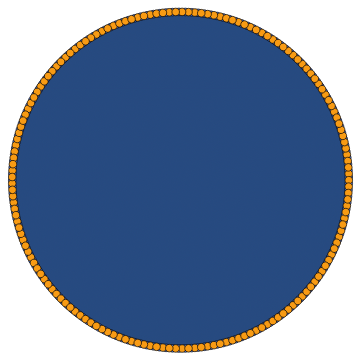
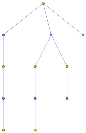
I can color the vertices of a random sample of bipartite graphs:
In[]:=
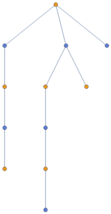
RandomSample[GraphData["Bipartite"],30]
Out[]=
{Foster674A,{KayakPaddle,{4,8,2}},{Antelope,{8,8}},{Tree,{12,295}},{Giraffe,{8,10}},{Gear,16},Foster554A,3P3,{FibonacciCube,13},{Tree,{12,164}},2P2+K1,{Tree,{11,84}},{Path,10},{CompleteBipartite,{6,20}},{CubicTransitive,68},{CompleteBipartite,{8,9}},{HexagonalGrid,{1,1,3}},{Firecracker,{7,3}},{Tree,{11,187}},Foster936A,{CompleteBipartite,{13,19}},{MongolianTent,{2,5}},{CompleteBipartite,{9,20}},{EdgeTransitive,{18,3}},{Tree,{11,58}},{Camel,{6,10}},{GeneralizedPetersen,{24,11}},Foster194A,{Tree,{10,64}},Foster880A}
In[]:=
PersistResourceFunction["ColorGraphVertices"]
Out[]=
Success
In[]:=
Select[GraphQ][ColorGraphVertices[GraphData[#]]&/@RandomSample[GraphData["Bipartite"],30]]
Out[]=
,
,
,
,
,
,
,
,
,
,
,
,
,
,
,
,
,
,
,
,
,
,
,
,
,

,
,
,
,
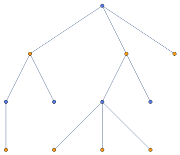
Exercise 49
Exercise 49
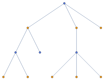
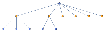
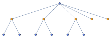
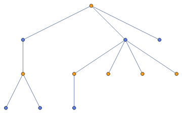
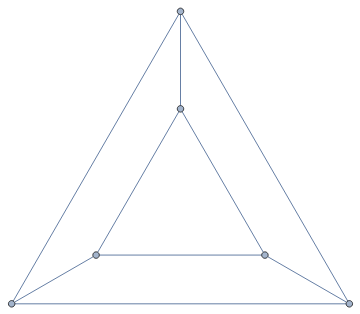
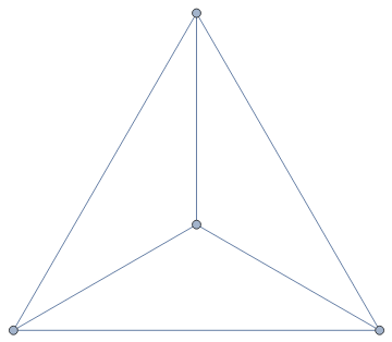
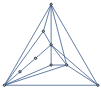
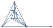
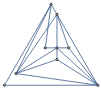
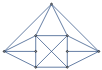
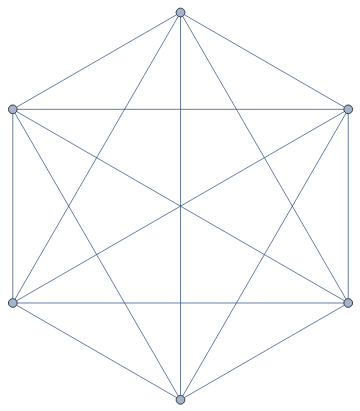
Draw diagrams of all the cubic graphs with at most 6 vertices:
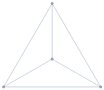
In[]:=
GraphData["Cubic"]
Out[]=
In[]:=
Select[VertexCount[GraphData[#]]<=6&][GraphData["Cubic"]]
Out[]=
{{Prism,3},TetrahedralGraph,UtilityGraph}
In[]:=
GraphData/@Select[VertexCount[GraphData[#]]<=6&][GraphData["Cubic"]]
Out[]=
,
,
Exercise 50
Exercise 50
Exercise 55
Exercise 55
Note
Note
A lot of the exercises are hard and involve proofs and higher mathematical thinking as can be seen in my difficulty with the previous problem with holonomic difference root objects and bipartite graphs, so I’m going to skip to the exercises I can use Mathematica on.
Exercise 83
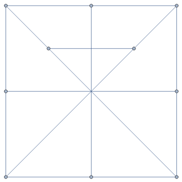
Exercise 83
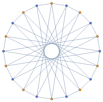
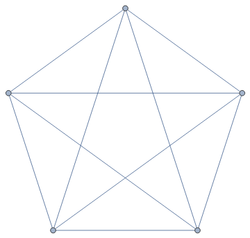
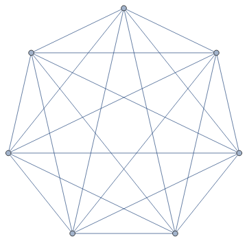
Draw the graph .
L()
K
5
This is the graph complement of the line graph of the complete graph of 5.
In[]:=
GraphComplement[LineGraph[CompleteGraph[5]]]
Out[]=
Transform the graph into a simpler form:
In[]:=
CanonicalGraph[GraphComplement[LineGraph[CompleteGraph[5]]]]
Out[]=
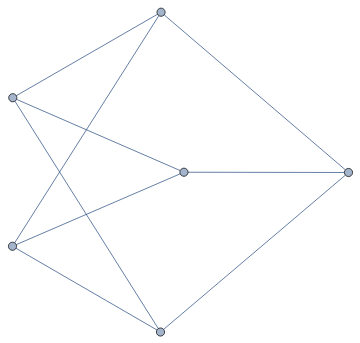
I think this is isomorphic to the Petersen graph.
In[]:=
IsomorphicGraphQ[CanonicalGraph[GraphComplement[LineGraph[CompleteGraph[5]]]],PetersenGraph[]]
Out[]=
True
I learned equals the Petersen graph.
L()
K
5
Exercise 84
Exercise 84
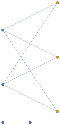
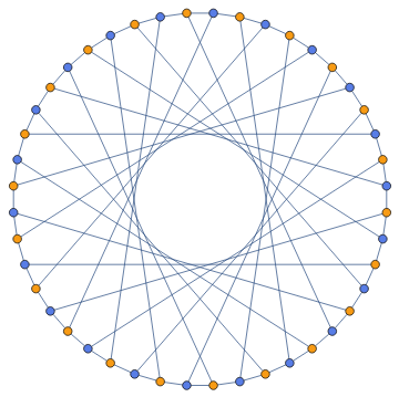
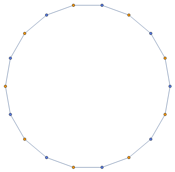
Is self-complementary?
L()
K
3,3
Find all known self-complementary graphs:
In[]:=
AssociationMap[GraphData,GraphData["SelfComplementary"]]
Out[]=
BullGraph
,{Circulant,{13,{1,2,4}}}
,{Circulant,{17,{1,2,3,6}}}
,{Circulant,{17,{1,2,3,7}}}

,{Circulant,{17,{1,3,4,5}}}

,{Cycle,5}

,{GeneralizedQuadrangle,{2,1}}
,{JohnsonSkeleton,26}

,{Paley,13}

,{Paley,17}

,{Paley,25}

,{Paley,29}

,{Paley,37}

,{Paley,41}

,{Paley,49}
,{Paley,53}

,{Paley,61}

,{Paley,73}

,{Paley,81}

,{Paley,89}

,{Paley,97}

,{Paley,101}

,{Paley,109}
,{Paley,113}

,{Paley,121}

,{Paley,125}

,{Paley,137}

,{Paley,149}

,{Paley,157}
,{Paley,169}

,{Path,4}

,{Quartic,{9,2}}

,{Quartic,{9,8}}
,{Quartic,{9,11}}

,{SelfComplementary,{8,1}}
,{SelfComplementary,{8,3}}
,{SelfComplementary,{8,4}}

,{SelfComplementary,{8,5}}

,{SelfComplementary,{8,6}}

,{SelfComplementary,{8,7}}

,{SelfComplementary,{8,8}}

,{SelfComplementary,{8,10}}

,{SelfComplementary,{9,1}}

,{SelfComplementary,{9,2}}

,{SelfComplementary,{9,3}}
,{SelfComplementary,{9,4}}

,{SelfComplementary,{9,5}}
,{SelfComplementary,{9,6}}
,{SelfComplementary,{9,7}}

,{SelfComplementary,{9,8}}
,{SelfComplementary,{9,9}}

,{SelfComplementary,{9,10}}

,{SelfComplementary,{9,11}}

,{SelfComplementary,{9,12}}
,{SelfComplementary,{9,13}}

,{SelfComplementary,{9,14}}

,{SelfComplementary,{9,15}}

,{SelfComplementary,{9,16}}

,{SelfComplementary,{9,17}}

,{SelfComplementary,{9,18}}

,{SelfComplementary,{9,19}}

,{SelfComplementary,{9,20}}
,{SelfComplementary,{9,21}}

,{SelfComplementary,{9,22}}
,{SelfComplementary,{9,23}}
,{SelfComplementary,{9,26}}
,{SelfComplementary,{9,27}}

,{SelfComplementary,{9,28}}
,{SelfComplementary,{9,29}}

,{SelfComplementary,{9,30}}
,{SelfComplementary,{9,31}}

,{SelfComplementary,{9,32}}
,{SelfComplementary,{9,34}}
,{SelfComplementary,{9,35}}
,SingletonGraph

,{Sun,4}


In[]:=
SelfComplementaryGraphQ//ClearAllSelfComplementaryGraphQ[graph_?GraphQ]:=IsomorphicGraphQ[graph,GraphComplement[graph]]
In[]:=
SelfComplementaryGraphQ[LineGraph[CompleteGraph[{3,3}]]]
Out[]=
True
In[]:=
LineGraph[CompleteGraph[{3,3}]]
Out[]=
In[]:=
GraphComplement[LineGraph[CompleteGraph[{3,3}]]]
Out[]=
In[]:=
IsomorphicGraphQ[GraphComplement[LineGraph[CompleteGraph[{3,3}]]],LineGraph[CompleteGraph[{3,3}]]]
Out[]=
True
The answer is that is self-complementary.
L()
K
3,3
The book says the answer is true. I originally got this wrong because I compared the graph and its complement with == instead of IsomorphicGraphQ.
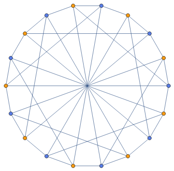
Exercise 87
Exercise 87
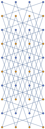
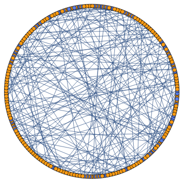
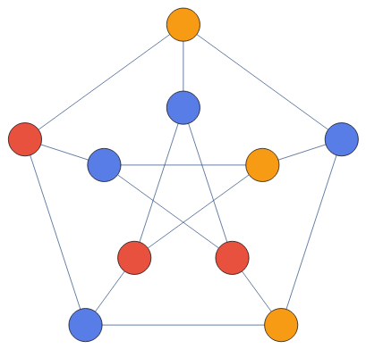
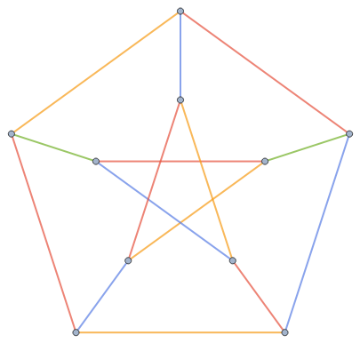
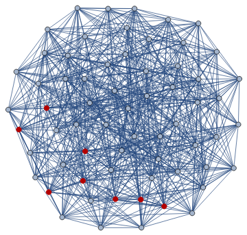
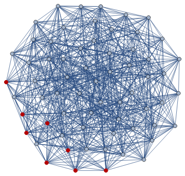
Is the Petersen graph (a) 3-colorable (b) 3-edge-colorable?
In[]:=
GraphData["PetersenGraph","ChromaticNumber"]
Out[]=
3
In[]:=
GraphData["PetersenGraph","EdgeChromaticNumber"]
Out[]=
4
Yes to a, no to b.
In[]:=
ColorGraphVertices[PetersenGraph[],ImageSize->Large,VertexSize->Large]
Out[]=
In[]:=
PersistResourceFunction[{"ColorGraphEdges"}]
Out[]=
Success
In[]:=
ColorGraphEdges[PetersenGraph[],ImageSize->Large,EdgeStyle->{Thick}]
Out[]=
Exercise 88
Exercise 88
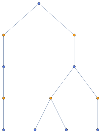
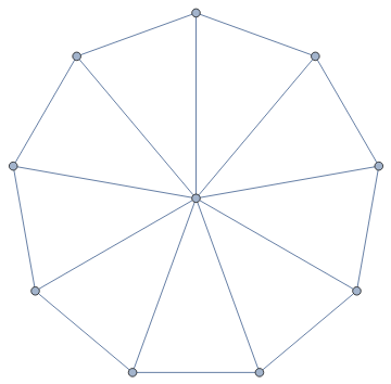
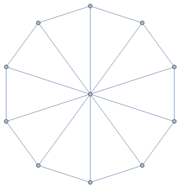
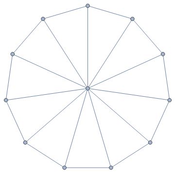
The graph =— is called the wheel with spokes, when . How many cycles does it contain as subgraphs?
W
n
K
1
C
n
n
n>=3
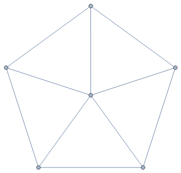
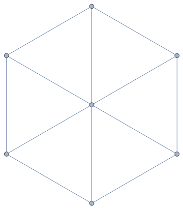
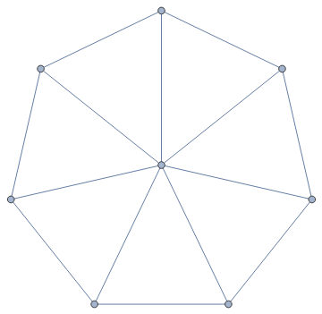
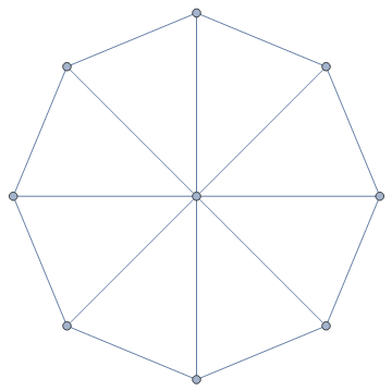
In[]:=
WheelGraph/@Range[12]
Out[]=
,

,
,
,

,
,
,
,
,
,
,
In[]:=
FindFundamentalCycles[WheelGraph[7]]
Out[]=
{{71,16,67},{61,15,56},{51,14,45},{41,13,34},{71,12,27},{31,12,23}}
In[]:=
Length[FindFundamentalCycles[WheelGraph[7]]]
Out[]=
6
Find all cycles of wheel graph 7.
In[]:=
FindCycle[WheelGraph[7],Infinity,All]
Out[]=
{{13,34,41},{14,45,51},{27,71,12},{23,31,12},{15,56,61},{17,76,61},{13,32,27,71},{13,34,45,51},{51,17,76,65},{23,34,41,12},{12,27,76,61},{14,45,56,61},{14,43,32,27,71},{54,41,17,76,65},{27,76,65,51,12},{23,34,45,51,12},{13,32,27,76,61},{13,34,45,56,61},{17,72,23,34,45,51},{51,13,32,27,76,65},{54,43,31,17,76,65},{54,43,32,27,76,65},{27,76,65,54,41,12},{12,23,34,45,56,61},{14,43,32,27,76,61},{51,14,43,32,27,76,65},{54,41,13,32,27,76,65},{27,76,65,54,43,31,12},{23,34,45,56,67,71,12},{15,54,43,32,27,76,61},{17,72,23,34,45,56,61}}
In[]:=
Length[FindCycle[WheelGraph[7],Infinity,All]]
Out[]=
31
In[]:=
Table[Length[FindCycle[WheelGraph[i],Infinity,All]],{i,3,18}]
Out[]=
{2,7,13,21,31,43,57,73,91,111,133,157,183,211,241,273}
In[]:=
FindSequenceFunction[Table[Length[FindCycle[WheelGraph[i],Infinity,All]],{i,3,18}]]
Out[]=
Donald Knuth doesn’t give a particular answer for this.
Exercise 91
Exercise 91
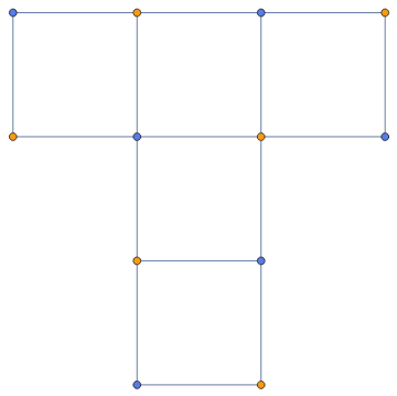
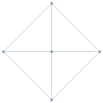
Draw diagrams for the 4-vertex graphs (a)
K
2
□K
2
The symbol □ represents the Cartesian graph product.
In[]:=
GraphProduct[CompleteGraph[2],CompleteGraph[2]]
Out[]=

(b) ⊗. The symbol ⊗ represents the juxtaposition, or direct sum of two graphs. I think I have the right function.
K
2
K
2
In[]:=
GraphDisjointUnion[CompleteGraph[2],CompleteGraph[2]]
Out[]=
Later on the symbol ⊗ is also used for the conjunction or direct product. I’m not sure if this is implemented in Mathematica or not yet.
In[]:=
GraphProduct[CompleteGraph[2],CompleteGraph[2],"Conormal"]
Out[]=

(c) symbol. Mathematica doesn’t support the next symbol, which is like a square with an X through its center, similar to the tensor product symbol used in part b but with a square instead of a circle.
K
2
K
2
I’m going to move onto another exercise because I’m not sure which graph product to use.
Exercise 124
Exercise 124
What is the chromatic number of the Chvàtal graph, Fig. 2(f)?
In[]:=
GraphData["ChvatalGraph","ChromaticNumber"]
Out[]=
4
Color the nodes:
In[]:=
ColorGraphVertices[GraphData["ChvatalGraph"],ImageSize->Large,VertexSize->Large]
Out[]=
Exercise 129
Exercise 129
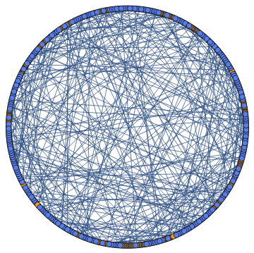
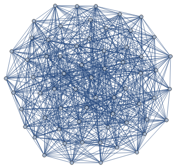
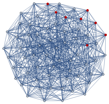
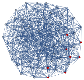
Describe the maximal cliques of the 8x8 queen graph (37).
In[]:=
GraphData[{"Queen",{8,8}}]
Out[]=
In[]:=
GraphData[{"Queen",{8,8}},"MaximumCliques"]
Out[]=
{{1,2,3,4,5,6,7,8},{1,9,17,25,33,41,49,57},{1,10,19,28,37,46,55,64},{2,10,18,26,34,42,50,58},{3,11,19,27,35,43,51,59},{4,12,20,28,36,44,52,60},{5,13,21,29,37,45,53,61},{6,14,22,30,38,46,54,62},{7,15,23,31,39,47,55,63},{8,15,22,29,36,43,50,57},{8,16,24,32,40,48,56,64},{9,10,11,12,13,14,15,16},{17,18,19,20,21,22,23,24},{25,26,27,28,29,30,31,32},{33,34,35,36,37,38,39,40},{41,42,43,44,45,46,47,48},{49,50,51,52,53,54,55,56},{57,58,59,60,61,62,63,64}}
In[]:=
HighlightGraph[GraphData[{"Queen",{8,8}}],#]&/@GraphData[{"Queen",{8,8}},"MaximumCliques"]
Out[]=
,
,
,
,

,
,
,
,

,
,
,
,
,
,
,
,
,
The book says 310 maximal cliques which is different from the answer from GraphData, so I’m confused.
Exercise 130
Exercise 130
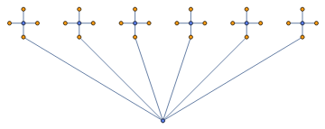
How many maximal cliques are in a complete k-partite graph?
I will try FindSequenceFunction.
In[]:=
Names["*clique*",IgnoreCase->True]
Out[]=
{FindClique,FindKClique}
In[]:=
Information/@Names["*clique*",IgnoreCase->True]
Out[]=
,
In[]:=
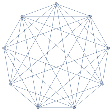
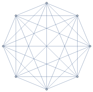
CompleteGraph[#]&/@Range[9]
Out[]=
,

,

,

,
,
,
,
,

In[]:=
FindClique[CompleteGraph[5],Infinity,All]
Out[]=
{{1,2,3,4,5}}
In[]:=
FindClique[CompleteGraph[#],Infinity,All]&/@Range[7]
Out[]=
{{{1}},{{1,2}},{{1,2,3}},{{1,2,3,4}},{{1,2,3,4,5}},{{1,2,3,4,5,6}},{{1,2,3,4,5,6,7}}}
I looks like a complete graph has just one maximal clique.
Exercise 132
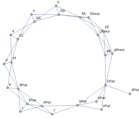
Exercise 132
I tried to finish entering a graph manually and it was taking too much time so I gave up.
There’s a picture of a graph and I’m asked to determine several properties.
I was trying to be careful as I entered the graph into Mathematica not to duplicate an edge, but then I realized that if I duplicated an edge I could just use SimpleGraph to get the underlying graph.
In[]:=
SimpleGraph@Graph[{AA<->b,AA<->fSharp,AA<->cSharp,AA<->DD,AA<->EE,DD<->fSharp,DD<->b,DD<->e,DD<->GG,GG<->e,GG<->b,GG<->a,GG<->CC,CC<->e,CC<->a,CC<->d,CC<->FF,FF<->a,FF<->d,FF<->g,FF<->BFlat,BFlat<->d,BFlat<->c,BFlat<->g,BFlat<->EFlat,EFlat<->AFlat,EFlat<->f,EFlat<->c,EFlat<->g,AFlat<->c,AFlat<->f,AFlat<->BFlat,AFlat<->DFlat,DFlat<->f,DFlat<->bFlat,DFlat<->eFlat,DFlat<->GFlat,GFlat<->eFlat,GFlat<->bFlat,GFlat<->dFlat,GFlat<->BB,GFlat<->gSharp,BB<->EE,EE<->cSharp,EE<->fSharp,EE<->gSharp,gSharp<->BB,gSharp<->cSharp,cSharp<->fSharp,cSharp<->BB,AFlat<->DFlat,DFlat<->f},VertexLabels->Automatic,ImageSize->Large]
Out[]=
In[]:=
SimpleGraphQ[SimpleGraph@Graph[{AA<->b,AA<->fSharp,AA<->cSharp,AA<->DD,AA<->EE,DD<->fSharp,DD<->b,DD<->e,DD<->GG,GG<->e,GG<->b,GG<->a,GG<->CC,CC<->e,CC<->a,CC<->d,CC<->FF,FF<->a,FF<->d,FF<->g,FF<->bFlat,bFlat<->d,bFlat<->c,bFlat<->g,bFlat<->eFlat,eFlat<->aFlat,eFlat<->f,eFlat<->c,eFlat<->g,aFlat<->c,aFlat<->f,aFlat<->bFlat,aFlat<->dFlat,dFlat<->f,dFlat<->bFlat,dFlat<->eFlat,dFlat<->gFlat,gFlat<->eFlat,gFlat<->bFlat,gFlat<->dFlat},VertexLabels->Automatic,GraphLayout->"TutteEmbedding"]]
Out[]=
True
Order
Order
Conclusion
Conclusion
I was able to solve several exercises in TAOCP with Mathematica.