CITE THIS NOTEBOOK: Characterization of multiway sequential cellular automata by Margaux Wong. Wolfram Community FEB 25 2023.
This essay was written by Margaux Wong as part of the Wolfram Emerging Leaders Program, which is a 4-month long, project-based program designed for gifted high school students to take a deep dive into a topic of their choice. Students work remotely in small groups or individually to take their project from ideation to completion, with the guidance of Wolfram experts. Wolfram Emerging Leaders Program participants are selected from the Wolfram High School Summer Camp, which is open to talented, STEM-oriented students age 17 and under.
Abstract
Abstract
Cellular Automata are used to model rule based evolutionary systems with unitary, fixed rules applied to an entire generation at a time. A new type of cellular automata using sequential updating with more than one rule for each input sequence is studied. These Multiway Sequential Cellular Automata (MSCA) can model complex systems with multiple branching rule sets where states propagate through the system. Potential applications include modeling aspects of quantum spin chains. This study examines two-block, two-rule MSCA using machine learning to classify 7776 resulting state graphs into 14 classes. Analytical data is used to not only characterize these classes of graphs but to investigate the role of initial conditions and rule sets in these state graphs.
Introduction
Introduction
The Quantum World
The Quantum World
Quantum field theory (QFT) studies the theoretical synthesis of classical field theory, special relativity, and quantum mechanics to model the physical behavior of subatomic particles as well as quasi-particles in condensed matter physics. [5] A fundamental aspect of quantum physics is its non-deterministic nature, which stems from Heisenberg’s uncertainty principle. The contrast between Bohr’s classical model of the atom and the Electron Cloud Model, which considers the uncertainty of the position and momentum of an electron, is a common example of this difference between deterministic classical physics and non-deterministic quantum physics. Similar to the model of an atom, enhancing our understanding of the universe relies on both classical and quantum models of physical mechanics.
Multiway Sequential Cellular Automata (MSCA), the subject of this study, has the potential for modeling simple quantum spin chains. These quantum spin chains enjoy short-range interactions that fit well with the propagating nature of MSCA while the multiway aspect allows for the modeling of complex behaviors.
Multiway Sequential Cellular Automata (MSCA), the subject of this study, has the potential for modeling simple quantum spin chains. These quantum spin chains enjoy short-range interactions that fit well with the propagating nature of MSCA while the multiway aspect allows for the modeling of complex behaviors.
Multiway Sequential Cellular Automata
Multiway Sequential Cellular Automata
Cellular automata (CA) are arrays of cells defined by an initial state and a list of evolutionary rules. In the binary state case, the initial state can be modeled as a row of black and white cells or zeroes and ones. CA rules define how a row of black and white cells are transformed into a new row of black and white cells. Each new cell’s value is based on values of the previous state of the array only. One common representation is to display these rows consecutively forming a grid of black and white cells. This two-dimensional grid thus shows the evolution of the pattern over successive application of the rules.
Sequential CA differ from standard CA in the application of rules on the current state. For sequential CA, blocks of cells to which the rules are applied overlap by 1 or more cells and for each row, only 1 block of cells is transformed while the rest of the cells remain constant. Thus each new row does not represent a complete generation, only one step of one generation. Then the next block of cells is transformed based on this newly transformed row. A generation is complete when all cells in the row have been transformed. Thus, for sequential CA, a cell impacts not only its direct successors but the successors of its neighbor providing a propagation of effects. A “generation of evolution” then also consists of several rows instead of one as each application of the rule set to one block of cells generates another row.
Additional complexity can be added to sequential CA through the use of multiway rules. Multiway CA evolve according to 2 or more sets of rules. Thus, for any given state, there are several different possible outcomes. These different evolutionary paths can be represented in a multiway graph.
Evolutionary Graphs
Evolutionary Graphs
M-type MSCA Rules
M-type MSCA Rules
possibles=Flatten[Table[{{a,b},{c,d}},{a,{0,1}},{b,{0,1}},{c,{0,1}},{d,{0,1}}],3];ww=Subsets[Partition[possibles,4][[1]],{2}];wb=Subsets[Partition[possibles,4][[2]],{2}];bw=Subsets[Partition[possibles,4][[3]],{2}];bb=Subsets[Partition[possibles,4][[4]],{2}];mListRules=Flatten[Table[Join[q,x,y,z],{q,ww},{x,wb},{y,bw},{z,bb}],3];mRules=Table[Association[{0,0}->{n[[1]][[2]],n[[2]][[2]]},{0,1}->{n[[3]][[2]],n[[4]][[2]]},{1,0}->{n[[5]][[2]],n[[6]][[2]]},{1,1}->{n[[7]][[2]],n[[8]][[2]]}],{n,mListRules}];
Evolutionary Graph Example
Evolutionary Graph Example
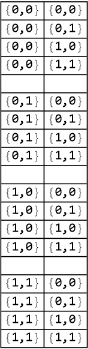
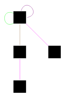
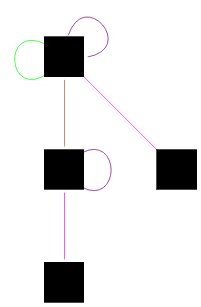
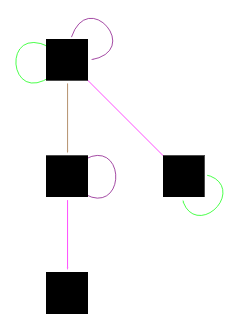
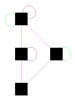
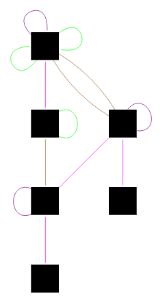
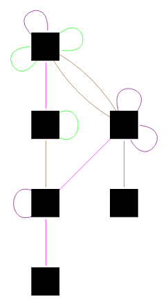
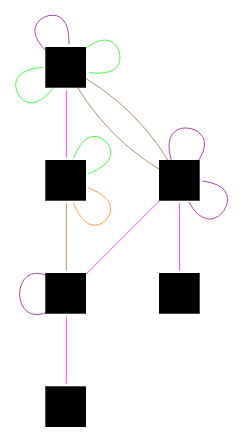
Starting with an initial condition of {0,1,1} and rule M1044, an example evolution would look as follows.
In[]:=
ruledRule1044={{0,0}->{0,1},{0,0}->{1,1},{0,1}->{0,1},{0,1}->{1,1},{1,0}->{1,0},{1,0}->{1,1},{1,1}->{1,0},{1,1}->{1,1}};
In[]:=
colorAssociation=<| 1->Blue, 2->Cyan, 3->Green, 4->Brown, 5->Orange, 6->Red, 7->Magenta, 8->Purple|>;
In[]:=
stateAssociation=<|{0,1,1}->1,{1,1,1}->2,{0,1,0}->3,{1,1,0}->4,{1,0,0}->5,{1,0,1}->6|>;
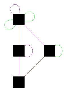
myGraphList={};AppendTo[myGraphList,{{0,1,1}->{0,1,1},{0,1}->{0,1}}];myGraph=EdgeTaggedGraph[ Table[Style[stateAssociation[Flatten[Keys[myGraphListRelationship[[1]]]]]->stateAssociation[Flatten[Values[myGraphListRelationship[[1]]]]],Directive[colorAssociation[Flatten[Position[ruledRule1044,myGraphListRelationship[[2]]]][[1]]],Small],Arrowheads[0.012]],{myGraphListRelationship,myGraphList}], VertexStyle->Black, VertexSize->Large, VertexShapeFunction->"Square"]
Out[]=

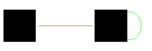
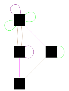
AppendTo[myGraphList,{{0,1,1}->{1,1,1},{0,1}->{1,1}}];myGraph=EdgeTaggedGraph[ Table[Style[stateAssociation[Flatten[Keys[myGraphListRelationship[[1]]]]]->stateAssociation[Flatten[Values[myGraphListRelationship[[1]]]]],Directive[colorAssociation[Flatten[Position[ruledRule1044,myGraphListRelationship[[2]]]][[1]]],Small],Arrowheads[0.012]],{myGraphListRelationship,myGraphList}], VertexStyle->Black, VertexSize->Large, VertexShapeFunction->"Square"]
Out[]=
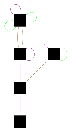
In[]:=
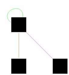
AppendTo[myGraphList,{{0,1,1}->{0,1,0},{1,1}->{1,0}}];myGraph=EdgeTaggedGraph[ Table[Style[stateAssociation[Flatten[Keys[myGraphListRelationship[[1]]]]]->stateAssociation[Flatten[Values[myGraphListRelationship[[1]]]]],Directive[colorAssociation[Flatten[Position[ruledRule1044,myGraphListRelationship[[2]]]][[1]]],Small],Arrowheads[0.012]],{myGraphListRelationship,myGraphList}], VertexStyle->Black, VertexSize->Large, VertexShapeFunction->"Square"]
Out[]=
In[]:=
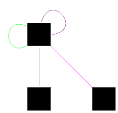
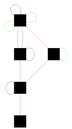
AppendTo[myGraphList,{{0,1,1}->{0,1,1},{1,1}->{1,1}}];myGraph=EdgeTaggedGraph[ Table[Style[stateAssociation[Flatten[Keys[myGraphListRelationship[[1]]]]]->stateAssociation[Flatten[Values[myGraphListRelationship[[1]]]]],Directive[colorAssociation[Flatten[Position[ruledRule1044,myGraphListRelationship[[2]]]][[1]]],Small],Arrowheads[0.012]],{myGraphListRelationship,myGraphList}], VertexStyle->Black, VertexSize->Large, VertexShapeFunction->"Square"]
Out[]=
In[]:=
AppendTo[myGraphList,{{1,1,1}->{1,1,0},{1,1}->{1,0}}];myGraph=EdgeTaggedGraph[ Table[Style[stateAssociation[Flatten[Keys[myGraphListRelationship[[1]]]]]->stateAssociation[Flatten[Values[myGraphListRelationship[[1]]]]],Directive[colorAssociation[Flatten[Position[ruledRule1044,myGraphListRelationship[[2]]]][[1]]],Small],Arrowheads[0.012]],{myGraphListRelationship,myGraphList}], VertexStyle->Black, VertexSize->Large, VertexShapeFunction->"Square"]
Out[]=
In[]:=
AppendTo[myGraphList,{{1,1,1}->{1,1,1},{1,1}->{1,1}}];myGraph=EdgeTaggedGraph[ Table[Style[stateAssociation[Flatten[Keys[myGraphListRelationship[[1]]]]]->stateAssociation[Flatten[Values[myGraphListRelationship[[1]]]]],Directive[colorAssociation[Flatten[Position[ruledRule1044,myGraphListRelationship[[2]]]][[1]]],Small],Arrowheads[0.012]],{myGraphListRelationship,myGraphList}], VertexStyle->Black, VertexSize->Large, VertexShapeFunction->"Square"]
Out[]=
(*Generation2*)AppendTo[myGraphList,{{0,1,0}->{0,1,0},{0,1}->{0,1}}];myGraph=EdgeTaggedGraph[ Table[Style[stateAssociation[Flatten[Keys[myGraphListRelationship[[1]]]]]->stateAssociation[Flatten[Values[myGraphListRelationship[[1]]]]],Directive[colorAssociation[Flatten[Position[ruledRule1044,myGraphListRelationship[[2]]]][[1]]],Small],Arrowheads[0.012]],{myGraphListRelationship,myGraphList}], VertexStyle->Black, VertexSize->Large, VertexShapeFunction->"Square"]
Out[]=
In[]:=
AppendTo[myGraphList,{{0,1,0}->{1,1,0},{0,1}->{1,1}}];myGraph=EdgeTaggedGraph[ Table[Style[stateAssociation[Flatten[Keys[myGraphListRelationship[[1]]]]]->stateAssociation[Flatten[Values[myGraphListRelationship[[1]]]]],Directive[colorAssociation[Flatten[Position[ruledRule1044,myGraphListRelationship[[2]]]][[1]]],Small],Arrowheads[0.012]],{myGraphListRelationship,myGraphList}], VertexStyle->Black, VertexSize->Large, VertexShapeFunction->"Square"]
Out[]=
In[]:=
AppendTo[myGraphList,{{0,1,1}->{0,1,1},{0,1}->{0,1}}];myGraph=EdgeTaggedGraph[ Table[Style[stateAssociation[Flatten[Keys[myGraphListRelationship[[1]]]]]->stateAssociation[Flatten[Values[myGraphListRelationship[[1]]]]],Directive[colorAssociation[Flatten[Position[ruledRule1044,myGraphListRelationship[[2]]]][[1]]],Small],Arrowheads[0.012]],{myGraphListRelationship,myGraphList}], VertexStyle->Black, VertexSize->Large, VertexShapeFunction->"Square"]
Out[]=
In[]:=
AppendTo[myGraphList,{{0,1,1}->{1,1,1},{0,1}->{1,1}}];myGraph=EdgeTaggedGraph[ Table[Style[stateAssociation[Flatten[Keys[myGraphListRelationship[[1]]]]]->stateAssociation[Flatten[Values[myGraphListRelationship[[1]]]]],Directive[colorAssociation[Flatten[Position[ruledRule1044,myGraphListRelationship[[2]]]][[1]]],Small],Arrowheads[0.012]],{myGraphListRelationship,myGraphList}], VertexStyle->Black, VertexSize->Large, VertexShapeFunction->"Square"]
Out[]=
In[]:=
AppendTo[myGraphList,{{1,1,0}->{1,0,0},{1,1}->{1,0}}];myGraph=EdgeTaggedGraph[ Table[Style[stateAssociation[Flatten[Keys[myGraphListRelationship[[1]]]]]->stateAssociation[Flatten[Values[myGraphListRelationship[[1]]]]],Directive[colorAssociation[Flatten[Position[ruledRule1044,myGraphListRelationship[[2]]]][[1]]],Small],Arrowheads[0.012]],{myGraphListRelationship,myGraphList}], VertexStyle->Black, VertexSize->Large, VertexShapeFunction->"Square"]
Out[]=
In[]:=
AppendTo[myGraphList,{{1,1,0}->{1,1,0},{1,1}->{1,1}}];myGraph=EdgeTaggedGraph[ Table[Style[stateAssociation[Flatten[Keys[myGraphListRelationship[[1]]]]]->stateAssociation[Flatten[Values[myGraphListRelationship[[1]]]]],Directive[colorAssociation[Flatten[Position[ruledRule1044,myGraphListRelationship[[2]]]][[1]]],Small],Arrowheads[0.012]],{myGraphListRelationship,myGraphList}], VertexStyle->Black, VertexSize->Large, VertexShapeFunction->"Square"]
Out[]=
In[]:=
AppendTo[myGraphList,{{1,1,1}->{1,0,1},{1,1}->{1,0}}];myGraph=EdgeTaggedGraph[ Table[Style[stateAssociation[Flatten[Keys[myGraphListRelationship[[1]]]]]->stateAssociation[Flatten[Values[myGraphListRelationship[[1]]]]],Directive[colorAssociation[Flatten[Position[ruledRule1044,myGraphListRelationship[[2]]]][[1]]],Small],Arrowheads[0.012]],{myGraphListRelationship,myGraphList}], VertexStyle->Black, VertexSize->Large, VertexShapeFunction->"Square"]
Out[]=
In[]:=
AppendTo[myGraphList,{{1,1,1}->{1,1,1},{1,1}->{1,1}}];myGraph=EdgeTaggedGraph[ Table[Style[stateAssociation[Flatten[Keys[myGraphListRelationship[[1]]]]]->stateAssociation[Flatten[Values[myGraphListRelationship[[1]]]]],Directive[colorAssociation[Flatten[Position[ruledRule1044,myGraphListRelationship[[2]]]][[1]]],Small],Arrowheads[0.012]],{myGraphListRelationship,myGraphList}], VertexStyle->Black, VertexSize->Large, VertexShapeFunction->"Square"]
Out[]=
In[]:=
AppendTo[myGraphList,{{0,1,0}->{0,1,0},{1,0}->{1,0}}];myGraph=EdgeTaggedGraph[ Table[Style[stateAssociation[Flatten[Keys[myGraphListRelationship[[1]]]]]->stateAssociation[Flatten[Values[myGraphListRelationship[[1]]]]],Directive[colorAssociation[Flatten[Position[ruledRule1044,myGraphListRelationship[[2]]]][[1]]],Small],Arrowheads[0.012]],{myGraphListRelationship,myGraphList}], VertexStyle->Black, VertexSize->Large, VertexShapeFunction->"Square"]
Out[]=
In[]:=
AppendTo[myGraphList,{{0,1,0}->{0,1,1},{1,0}->{1,1}}];myGraph=EdgeTaggedGraph[ Table[Style[stateAssociation[Flatten[Keys[myGraphListRelationship[[1]]]]]->stateAssociation[Flatten[Values[myGraphListRelationship[[1]]]]],Directive[colorAssociation[Flatten[Position[ruledRule1044,myGraphListRelationship[[2]]]][[1]]],Small],Arrowheads[0.012]],{myGraphListRelationship,myGraphList}], VertexStyle->Black, VertexSize->Large, VertexShapeFunction->"Square"]
Out[]=
In[]:=
AppendTo[myGraphList,{{1,1,0}->{1,1,0},{1,0}->{1,0}}];myGraph=EdgeTaggedGraph[ Table[Style[stateAssociation[Flatten[Keys[myGraphListRelationship[[1]]]]]->stateAssociation[Flatten[Values[myGraphListRelationship[[1]]]]],Directive[colorAssociation[Flatten[Position[ruledRule1044,myGraphListRelationship[[2]]]][[1]]],Small],Arrowheads[0.012]],{myGraphListRelationship,myGraphList}], VertexStyle->Black, VertexSize->Large, VertexShapeFunction->"Square"]
Out[]=
In[]:=
AppendTo[myGraphList,{{1,1,0}->{1,1,1},{1,0}->{1,1}}];myGraph=EdgeTaggedGraph[ Table[Style[stateAssociation[Flatten[Keys[myGraphListRelationship[[1]]]]]->stateAssociation[Flatten[Values[myGraphListRelationship[[1]]]]],Directive[colorAssociation[Flatten[Position[ruledRule1044,myGraphListRelationship[[2]]]][[1]]],Small],Arrowheads[0.012]],{myGraphListRelationship,myGraphList}], VertexStyle->Black, VertexSize->Large, VertexShapeFunction->"Square"]
Out[]=
In[]:=
AppendTo[myGraphList,{{1,0,0}->{1,0,1},{0,0}->{0,1}}];myGraph=EdgeTaggedGraph[ Table[Style[stateAssociation[Flatten[Keys[myGraphListRelationship[[1]]]]]->stateAssociation[Flatten[Values[myGraphListRelationship[[1]]]]],Directive[colorAssociation[Flatten[Position[ruledRule1044,myGraphListRelationship[[2]]]][[1]]],Small],Arrowheads[0.012]],{myGraphListRelationship,myGraphList}], VertexStyle->Black, VertexSize->Large, VertexShapeFunction->"Square"]
Out[]=
In[]:=
AppendTo[myGraphList,{{1,0,0}->{1,1,1},{0,0}->{1,1}}];myGraph=EdgeTaggedGraph[ Table[Style[stateAssociation[Flatten[Keys[myGraphListRelationship[[1]]]]]->stateAssociation[Flatten[Values[myGraphListRelationship[[1]]]]],Directive[colorAssociation[Flatten[Position[ruledRule1044,myGraphListRelationship[[2]]]][[1]]],Small],Arrowheads[0.012]],{myGraphListRelationship,myGraphList}], VertexStyle->Black, VertexSize->Large, VertexShapeFunction->"Square"]
Out[]=
In[]:=
AppendTo[myGraphList,{{1,0,1}->{1,0,1},{0,1}->{0,1}}];myGraph=EdgeTaggedGraph[ Table[Style[stateAssociation[Flatten[Keys[myGraphListRelationship[[1]]]]]->stateAssociation[Flatten[Values[myGraphListRelationship[[1]]]]],Directive[colorAssociation[Flatten[Position[ruledRule1044,myGraphListRelationship[[2]]]][[1]]],Small],Arrowheads[0.012]],{myGraphListRelationship,myGraphList}], VertexStyle->Black, VertexSize->Large, VertexShapeFunction->"Square"]
Out[]=
Data Generation and Machine Learning Classification
Data Generation and Machine Learning Classification
Two block MSCA rule sets which transform pairs of cells were examined using a novel implementation of this particular type of cellular automata. Previous implementation of the MSCA was for a specialized circular type. [1] In this implementation, the propagation ends at the end of each generation and does not propagate to the beginning of the row from the end. Multiway systems with two rules for each pair of cells were used. Since there are 4 possible cell pair values (0,0) (0,1) (1,0) (1,1) and two rules were specified for each, that results in 8 rules per case. Cell pair values were prohibited from remaining unchanged and the two multiway rules were required to be distinct. Therefore, for each cell pair value there were three possibilities for the first rule, i.e. the pair could be changed to any of the other three possible cell pair values. Since the rules had to be distinct, that left only two possibilities for the second rule. Thus, there were six possible combinations of rules for each of the four cell pair values, resulting in 1296 possible rule combinations in total.
Six different initial conditions (000100, 001110, 010110, 101011, 110011, 111001) were run through these 1296 possible rules, yielding 7776 cases. For each case, a states graph was made with each node representing a particular set of states connected by edges to show the progression through the nodes. The edges were colored to indicate which of the rules were applied to progress from one node to the next. Rules applied to (0,0) were colored blue/cyan, those applied to (0,1) were colored green/yellow, those applied to (1,0) were colored orange/red, and those applied to (1,1) were colored magenta/purple.
Graphs from two initial conditions, a total of 2592 cases, were examined to determine the unique graph classes. 14 different classes were identified. 1555 of these graphs or 20% of the total were used to form a training data set. The Wolfram machine learning function Classify[] was then used to classify the remaining 6221 graphs into the 14 predetermined classes. The 1037 graphs that had been hand classified but were not used for the training data were used to check the level of agreement between hand classification and the trained classifier function. Of these graphs, 88% were classified the same.
Graph Classes
Graph Classes
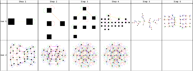
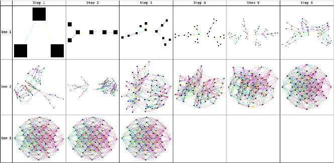
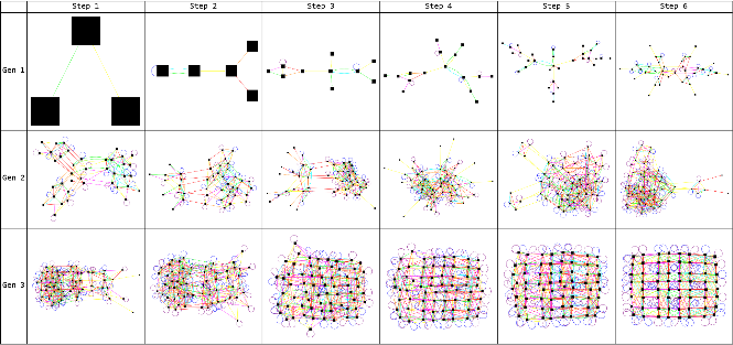
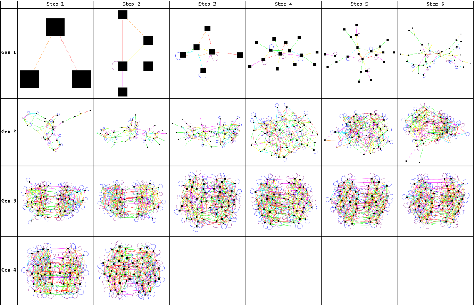
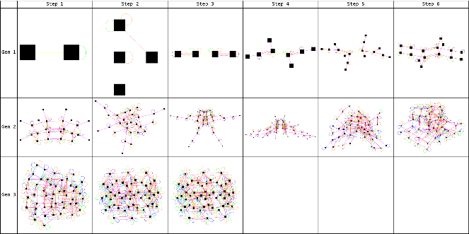
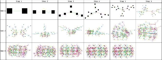
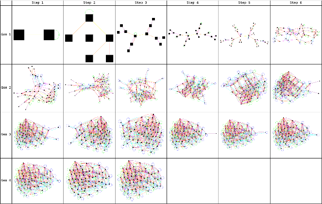
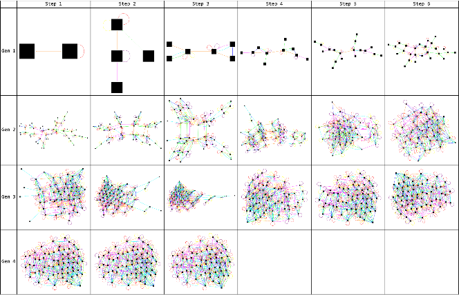
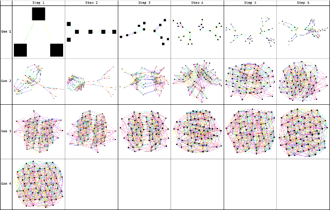
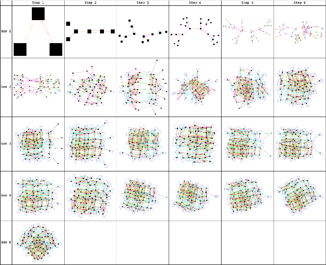
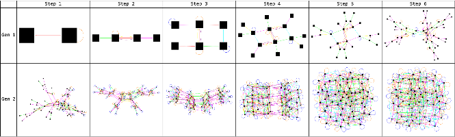
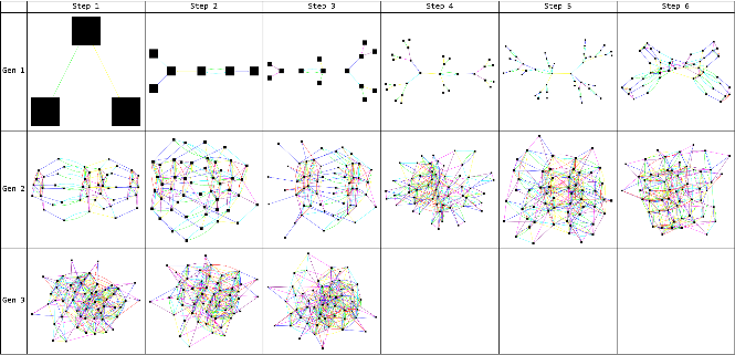
There are 14 classes of graphs. For each class, an exemplar is shown followed by a table displaying the evolution of the graph. Each row in the table shows a full generation of evolution, meaning the full row of cells has evolved once according to the predetermined rules. Each column within a row shows one step of evolution which is the application of the full rule set on one pair of cells.
Class 1 Graphs - Circles
Class 1 Graphs - Circles
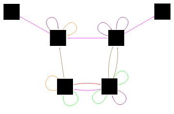
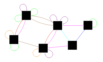
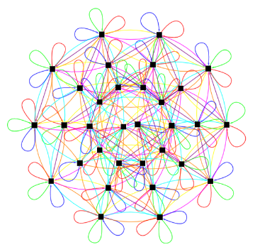
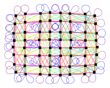
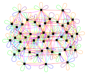
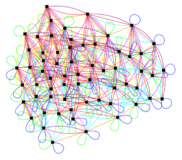
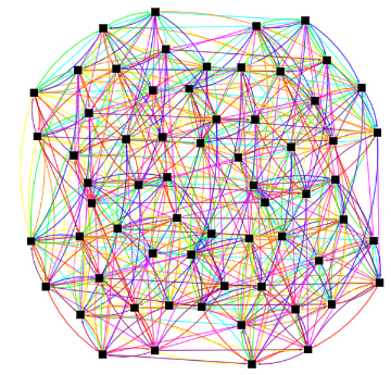
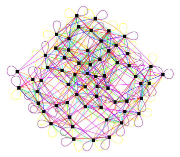
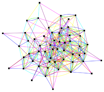
Class 1 graphs are circular and possess evenly distributed nodes on the outer ring. The image below is an exemplar of this class of graphs.
The following table shows the development of the exemplar graph for Class 1. The graph in generation 1, step 5 is noteworthy for its symmetry and bimodal nature. The graph converges by step 4 of the 2nd generation.
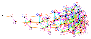
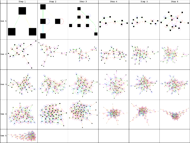
Class 2 Graphs - Footballs
Class 2 Graphs - Footballs
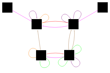
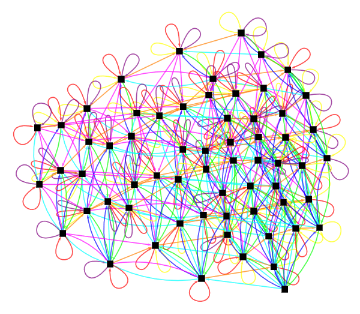
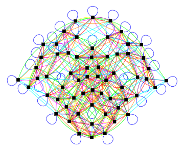
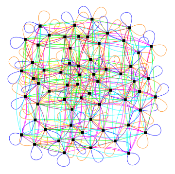
Class 2 graphs have symmetric nodes and are similar to the circles of Class 1 though slightly more oblong. The image below is an exemplar of this class of graphs.
The following table shows the development of the exemplar graph for Class 2. Note that the football shape has formed by step 6 of generation 2 although convergence does not occur until step 3 of generation 3.
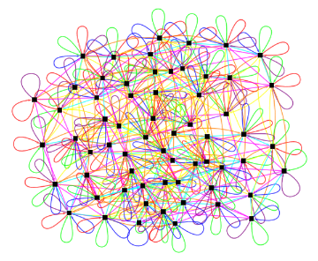
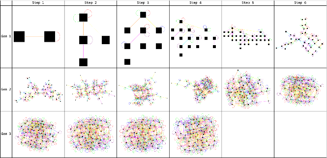
Class 3 Graphs - Rectangles
Class 3 Graphs - Rectangles
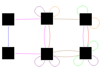
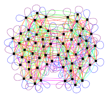
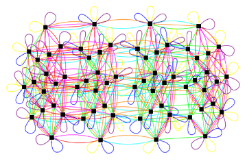
Class 3 graphs are rectangular and two-dimensional array of nodes. They consists of two types of columns that alternate. The image below is an exemplar of this class of graphs.
The following table shows the development of the exemplar graph for Class 3.
Class 4 Graphs - Bisectors
Class 4 Graphs - Bisectors
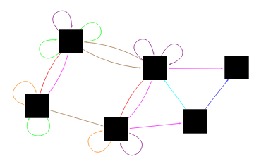
Class 4 graphs are bisectors and possess two clusters of nodes. The image below is an exemplar of this class of graphs.
The following table shows the development of the exemplar graph for Class 4.
Class 5 Graphs - Trisectors
Class 5 Graphs - Trisectors
Class 5 graphs are trisectors and possess three sectors of nodes. The image below is an exemplar of this class of graphs.
The following table shows the development of the exemplar graph for Class 5.
Class 6 Graphs - Quadsectors
Class 6 Graphs - Quadsectors
Class 6 graphs are quadsectors and possess four sectors of nodes. The image below is an exemplar of this class of graphs.
The following table shows the development of the exemplar graph for Class 6.
Class 7 Graphs - Fish
Class 7 Graphs - Fish
Class 7 graphs are asymmetric and have a shape reminiscent of a sunfish. The image below is a left facing exemplar of this class of graphs.
The following table shows the development of the left facing exemplar graph for Class 7.
The image below is a right facing exemplar of this class of graphs.
The following table shows the development of the right facing exemplar graph for Class 7.
Class 8 Graphs - Quadrectangles
Class 8 Graphs - Quadrectangles
Class 8 graphs have four subsections and a rectangular central section. The image below is an exemplar of this class of graphs.
The following table shows the development of the exemplar graph for Class 8.
Class 9 Graphs - Pseudo-footballs
Class 9 Graphs - Pseudo-footballs
Class 9 graphs are asymmetric and have a high density region of nodes in one section and an oblong character. The image below is an exemplar of this class of graphs.
The following table shows the development of the exemplar graph for Class 9.
Class 10 Graphs - Cubes
Class 10 Graphs - Cubes
Class 10 graphs have a cubic nature. The image below is an exemplar of this class of graphs.
The following table shows the development of the exemplar graph for Class 10.

Class 11 Graphs - Pseudo-Rectangles
Class 11 Graphs - Pseudo-Rectangles
Class 11 graphs appear to be distorted rectangles. The image below is an exemplar of this class of graphs.
The following table shows the development of the exemplar graph for Class 11.
Class 12 Graphs - Swordfish
Class 12 Graphs - Swordfish
Class 12 graphs are more linear than other classes with a cluster of nodes at one end. The image below is an exemplar of this class of graphs.
The following table shows the development of the exemplar graph for Class 12.
Class 13 Graphs - Closed Unknown
Class 13 Graphs - Closed Unknown
Class 13 graphs are graphs that do not fit the other classes with a number of loops indicating rules that sent a node back to itself. The image below is an exemplar of this class of graphs.
The following table shows the development of the exemplar graph for Class 13.
Class 14 Graphs - Open Unknown
Class 14 Graphs - Open Unknown
Class 14 graphs are graphs that do not fit the other classes and do not possess loops from rules that send a node back to itself. The image below is an exemplar of this class of graphs.
The following table shows the development of the exemplar graph for Class 14.
Graph Analysis
Graph Analysis
Graph Analytics
Graph Analytics
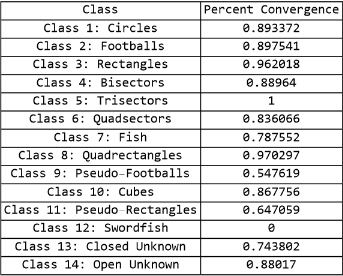
For each case, the multiway sequential cellular automata were allowed to run until either convergence was achieved or 5 full generations were calculated. Convergence was determined by examining the states after every step. If that specific state had been previously reached at the same step within a row, it was determined that the graph had converged as any further evolution would not yield any new paths on the graph. The table below shows the percent of convergence for each class of graphs. Class 5 (Trisectors) and 12 (Swordfish) had very few members, hence their outlier convergence numbers. It is interesting to note that of the other classes, the highest convergence rates are found in the rectangles, quadsectors, and quadrectangles which are highly related classes. The lowest rates of convergence are found in the pseudo-footballs and cubes.
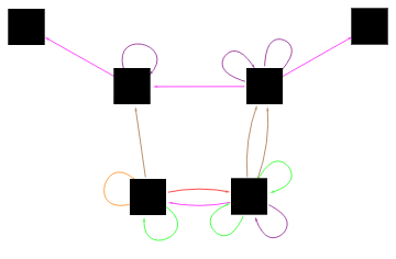
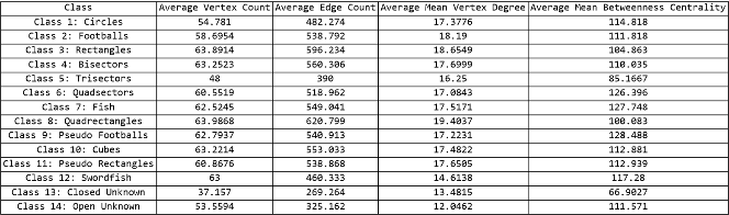
Analytical data was calculated for each of the 7776 graphs including vertex count, edge count, mean vertex degree, and mean betweenness centrality. For the evolutionary graph example shown at the beginning, the following analytical data can be calculated.
In[]:=
vertexCount=VertexCount[myGraph];edgeCount=EdgeCount[myGraph];meanVertexDegree=N[Mean[VertexDegree[myGraph]]];meanVertexInDegree=N[Mean[VertexInDegree[myGraph]]];meanBetweennessCentrality=N[Mean[BetweennessCentrality[myGraph]]];StringJoin["Vertex Count: ",ToString[vertexCount]]StringJoin["Edge Count: ",ToString[edgeCount]]StringJoin["Mean Vertex Degree: ",ToString[meanVertexDegree]]StringJoin["Mean Vertex In Degree: ",ToString[meanVertexInDegree]]StringJoin["Mean Betweenness Centrality: ",ToString[meanBetweennessCentrality]]
Out[]=
Vertex Count: 6
Out[]=
Edge Count: 24
Out[]=
Mean Vertex Degree: 8.
Out[]=
Mean Vertex In Degree: 4.
Out[]=
Mean Betweenness Centrality: 2.33333
An average value was calculated for each graphical measure for each of the 14 classes as shown in the table below. In all four measures, Class 13 (Closed Unknown) was an outlier and Class 14 (Open Unknown) was an outlier in three of the four measures. Class 5 (Trisectors) was also an outlier in all four measures though had very few members compared to the other 13 classes.
Histograms
Histograms
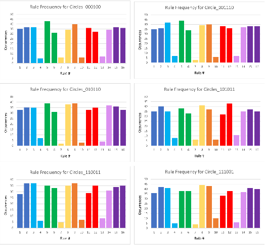
In order to examine the impact of specific rules on the ultimate form of the graph, rule frequencies were calculated for each class of graphs. Histograms were made of the rules used to generate the graphs in each class. The data was separated by initial condition to remove that variable from the data. Therefore, 6 histograms were created for each class of graphs, each corresponding to a different initial condition. The histograms were color coded to mimic the color coding of the rules in the graphs. The x-axis shows the rule number from the rule table in the section entitled MSCA Rules and the y-axis shows the number of graphs that were generated from a rule set containing that rule.
Histograms were analyzed for each class comparing all 6 initial conditions. A significant amount of similarity was found in 9 of the classes (circles, footballs, rectangles, bisectors, quadsectors, fish, quadrectangles, pseudo-footballs, pseudo-rectangles). The classes with more diversity in histograms were either very small classes (trisector with no members outside of training data, cube, and swordfish) or the catch-all classes (unknown open, unknown closed). Therefore, this analysis confirms that the rule set has a far greater impact on the shape of the final graph than the initial condition. An example set of these histograms for class 1 circles is shown below.
Histograms were analyzed for each class comparing all 6 initial conditions. A significant amount of similarity was found in 9 of the classes (circles, footballs, rectangles, bisectors, quadsectors, fish, quadrectangles, pseudo-footballs, pseudo-rectangles). The classes with more diversity in histograms were either very small classes (trisector with no members outside of training data, cube, and swordfish) or the catch-all classes (unknown open, unknown closed). Therefore, this analysis confirms that the rule set has a far greater impact on the shape of the final graph than the initial condition. An example set of these histograms for class 1 circles is shown below.
Histograms for Class 1 Circles for 6 different initial conditions
Histograms for Class 1 Circles for 6 different initial conditions
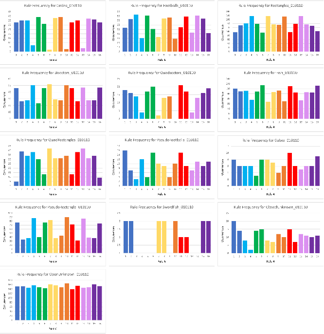
A comparison of the histograms for a single initial condition show some interesting properties as well. As all initial conditions had similar results, an analysis is performed on only one case (010110). It can be observed that the histogram for bisectors has many similarities to that of pseudo-footballs and pseudo-rectangles. While the scales are different, the bisector and pseudo-rectangle histograms are extremely similar on a relative basis. Compared to the histogram of pseudo-footballs, bisectors have higher relative occurrences of rule 7 and 13 but are otherwise well matched. Histograms of pseudo-footballs, in fact, have little resemblance to the histograms of footballs, despite similarities in the state graphs. Footballs, on the other hand, have histograms that are closest to that of circles. Both have relatively fewer occurrences of rules 4, 7, 10, and 13 with circles having extremely few occurrences of all four of these rules. Visually, footballs look like circles except they are oblong so the histogram similarity is not surprising. Quadsectors and fish also share many characteristics on their histograms with quadsectors having much more pronounced dips at rules 4, 7, 10, and 13. These are the same rules where dips occur in the histograms of circles and footballs. While the rest of the histograms differ between circles/footballs and quadsectors/fish, all four show have relatively few occurrences of rules 4, 7, 10, and 13. Finally, the histogram for quadrectangles seems to be an exaggerated version of the histogram for rectangles, underlining the close relationship between these classes.
A comparison of the histograms for a single initial condition show some interesting properties as well. As all initial conditions had similar results, an analysis is performed on only one case (010110). It can be observed that the histogram for bisectors has many similarities to that of pseudo-footballs and pseudo-rectangles. While the scales are different, the bisector and pseudo-rectangle histograms are extremely similar on a relative basis. Compared to the histogram of pseudo-footballs, bisectors have higher relative occurrences of rule 7 and 13 but are otherwise well matched. Histograms of pseudo-footballs, in fact, have little resemblance to the histograms of footballs, despite similarities in the state graphs. Footballs, on the other hand, have histograms that are closest to that of circles. Both have relatively fewer occurrences of rules 4, 7, 10, and 13 with circles having extremely few occurrences of all four of these rules. Visually, footballs look like circles except they are oblong so the histogram similarity is not surprising. Quadsectors and fish also share many characteristics on their histograms with quadsectors having much more pronounced dips at rules 4, 7, 10, and 13. These are the same rules where dips occur in the histograms of circles and footballs. While the rest of the histograms differ between circles/footballs and quadsectors/fish, all four show have relatively few occurrences of rules 4, 7, 10, and 13. Finally, the histogram for quadrectangles seems to be an exaggerated version of the histogram for rectangles, underlining the close relationship between these classes.
Histograms for different classes with the initial condition (010110)
Histograms for different classes with the initial condition (010110)
Histograms for different classes with the initial condition (010110)
Conclusion and Future Work
Conclusion and Future Work
A new form of cellular automata, multiway sequential cellular automata, which allows for propagation of effects, has been examined. A varied set of initial conditions was run through the entire group of 1296 possible rule sets for a two-block, two-rule MSCA. A classifier optimized for speed, accuracy, and memory was trained and then used to classify the resulting 7776 states graphs into 14 classes. These classes were analyzed to gain insight into the rules that yielded each class. Characteristics of the graphs of each class were also explored. It was determined that the relationship between rule frequency and class is governed by class and not by initial condition. Furthermore, the rule frequency has distinct characteristics for several of the classes. Convergence was also examined and while overall convergence rates were high, there were classes that were clear outliers.
More research is necessary to determine if the graphs that did not converge within 5 generations of evolution will converge with additional evolution time, and if so, if they will remain in their current class or morph into a different class. Correlations between specific rules and convergence rate also need to be examined. The distribution of color (representing specific rules) within each graph is another interesting area for future work as some graphs show concentrations of color while others show colors linked to specific graph features. Finally, expansion of the multiway system to more dimensions is a worthwhile extension.
More research is necessary to determine if the graphs that did not converge within 5 generations of evolution will converge with additional evolution time, and if so, if they will remain in their current class or morph into a different class. Correlations between specific rules and convergence rate also need to be examined. The distribution of color (representing specific rules) within each graph is another interesting area for future work as some graphs show concentrations of color while others show colors linked to specific graph features. Finally, expansion of the multiway system to more dimensions is a worthwhile extension.
Acknowledgements
Acknowledgements
I would like to thank Stephen Wolfram for the inspiration to work on this topic. I would like to thank James Boyd for invaluable technical mentorship and Rory Foulger for unbridled support.
References
References
1
.Wong, M. (2022, July). Multiway sequential cellular automata. https://community.wolfram.com/groups/-/m/t/2580859
2
.Boyd, J. (2022, June 6). Multicomputational Irreducibility. Wolfram Physics Project. https://www.wolframphysics.org/bulletins/2022/06/multicomputational-irreducibility/
3
.4
.Peskin, M. E., Schroeder, D. (1995). An Introduction to Quantum Field Theory (Avalon Publishing)
5
.Wolfram, S. (2002). A New Kind of Science. Wolfram Media.