As climate change and urbanization continue to intensify, an estimated 115 million individuals face heightened risks from wildfires. This escalating exposure highlights the need for accurate modeling tools to inform mitigation strategies. Thus, this project develops a cellular automaton (CA) framework to investigate spread dynamics and optimize fire suppressant placement. We generated landscapes made up of diverse patch types based on satellite imagery and elevation data, then create and apply a CA rule set to take into account wind, slope, moisture, radiation flux, and ember transport. Finally, we created a fire retardant deployment algorithm that leverages our simulation outputs to identify high risk zones and strategically allocate resources to suppress fires.
Introduction
Introduction
Merit for Using Cellular Automata in Modeling Wildfires
Merit for Using Cellular Automata in Modeling Wildfires
Many classical wildfire models, such as Rothermel’s, are limited to only calculating the rate of spread and cannot simulate fire propagation nor estimate burn area. To overcome these limitations, we implement a CA model which enables spatially explicit and time-evolving simulations of fire behavior. Since CA models are particularly well suited for heterogeneous terrains and capturing local interactions, that makes them ideal for this task.
Project Roadmap
Project Roadmap
01 Model Development: This section goes through the construction of our wildfire-spread model, starting with a brief introduction to cellular automata, the theoretical choice of cellular automata, and how it will be applied to 2D and 3D terrain.
02 Creating the Wildfire Spread Simulation: This section primarily implements the mechanics that go into modeling a wildfire: implementing patch properties, integrating satellite imagery, and creating the cellular automata rule for wildfire spread.
03 Modeling the 2D Wildfire Spread: This section focuses on modeling the 2D wildfire spread through plotting the terrain and running the 2D simulation.
04 Modeling the 3D Wildfire Spread: This section extends the 2D wildfire spread model into three dimensions through creating new functions to visualize and run the simulation in 3D.
05 Optimizing Fire Suppressant Placement: This section primarily implements an optimized fire suppressant algorithm
01. Model Development
01. Model Development
An Introduction to Cellular Automata
An Introduction to Cellular Automata
A cellular automaton (CA) is a discrete computational models consisting of a regular grid of cells, each existing in one of a finite number of states . The state of each cell evolves over discrete time steps according to a fixed set of rules that depend on the current states of the cell and its neighbors. In CA models, global patterns arise from local interactions without the need for centralized control or complex differential equations. Each cell's next state is determined solely by its current state and the states of cells within a defined neighborhood, typically the eight adjacent cells in a two-dimensional grid. This framework has been successfully applied across diverse fields, from Conway's Game of Life to traffic flow modeling, crystal growth simulations, and epidemic spread.
Adopting Cellular Automata
Adopting Cellular Automata
Having previously developed a cellular automata model for epidemiological disease spread, the transition to wildfire modeling leveraged the fundamental similarities between contagion dynamics in both systems. The model implements a grid-based system where each cell transitions between three primary states: unburned, burning, and burned—analogous to the susceptible-infected-recovered paradigm. The burning state incorporates a countdown mechanism for fuel-specific burn durations, while local spread rules calculate ignition probability based on heat from neighboring cells, modified by distance decay, slope multipliers, wind-driven ember transport, and terrain-specific properties like flammability and heat resistance.
A 2D and 3D Wildfire Simulation
A 2D and 3D Wildfire Simulation
We first create a 2D simulation, then move on to the 3D simulation. Running the model in 2D first is far cheaper computationally, exposes rule errors instantly, and lets us tune ignition probabilities or wind factors without rendering overhead. Once the 2D grid is stable, we reuse its state map as a texture/height pair for the 3D mesh, adding topographic realism without touching the underlying spread logic.
02. Creating the Wildfire Spread Simulation
02. Creating the Wildfire Spread Simulation
03. Modeling 2D Wildfire Spread
03. Modeling 2D Wildfire Spread
The goal of this section is to create a robust, visualized 2D simulation that serves as the foundation for the 3D system. In order to model the 3D system, we must first understand and be able to accurately represent fire spread in the 2D system. We first plot the 2D terrain then run the fire simulation.
Plotting the Terrain
Plotting the Terrain
Before we initialize the fires, we must first have the initial terrain; thus, we create the plotTerrainfunction.
This function primarily creates a colored grid plot from a 2D array based on the previously generated terrain grid from the initializeTerrainGrid function. Then, it applies the previously defined color scheme to the different elements of the array to create the grid .
In[]:=
plotTerrain[terrainGrid_,title_:""]:=ArrayPlot[terrainGrid,ColorRules->$terrainColorRules,Mesh->False,ImageSize->200,PlotLabel->title]
Plotting the Fire
Plotting the Fire
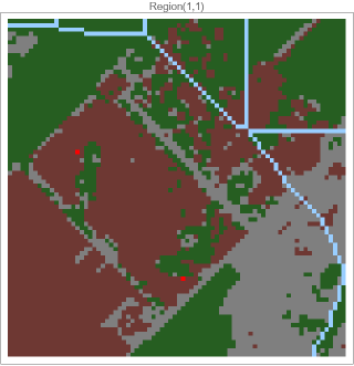
Then, the plotFirefunction is designed to visually represent the progression of a wildfire simulation by combining terrain data and fire status.
This function takes in 2D arrays : fireGrid, which encodes the first state of each cell, and terrainGrid, which represents the terrain type at each location . Within the function, a new grid called displayGrid is constructed using a Table and Which statement . If a cell is actively burning (values 1–10), it is assigned a corresponding display value from 11 to 20 to differentiate burn stages. Burned - out cells (value 11) are assigned a display value of 25. If a cell is unburned, its value is taken directly from the terrainGrid to preserve its terrain type . This processed grid is then visualized using ArrayPlot, with a predefined set of color rules to assign distinct colors to each fire and terrain state .
In[]:=
plotFire[fireGrid_,terrainGrid_,title_:""]:=Module[{displayGrid},displayGrid=Table[Which[fireGrid[[i,j]]>0&&fireGrid[[i,j]]<=10,10+fireGrid[[i,j]],fireGrid[[i,j]]==11,25,True,terrainGrid[[i,j]]],{i,Length[fireGrid]},{j,Length[fireGrid[[1]]]}];ArrayPlot[displayGrid,ColorRules->$firePlotColorRules,Mesh->False,ImageSize->400,PlotLabel->title]]
This function calls plotFire to every cell in the terrainGrid.
In[]:=
plotAllFireRegions[terrainGrids_,fireGrids_,numRows_,numCols_]:=Module[{plots},plots=Table[plotFire[fireGrids[[i,j]],terrainGrids[[i,j]],"Region("<>ToString[i]<>","<>ToString[j]<>")"],{i,numRows},{j,numCols}];Grid[plots,Spacings->{1,1}]]
Running the 2D Simulation
Running the 2D Simulation
Helper Functions
Helper Functions
The following functions are used for identifying the burnt, unburnt, and burning positions of cells on the grid.
In[]:=
getUnburnedPositions[fireGrid_]:=Position[fireGrid,0];getBurningPositions[fireGrid_]:=Position[fireGrid,y_/;1<=y<=10];getBurnedPositions[fireGrid_]:=Position[fireGrid,11];
The following functions are used for counting the number of burnt, unburnt, and burning positions of cells on the grid.
In[]:=
countUnburned[fireGrid_]:=Count[Flatten[fireGrid],0];countBurning[fireGrid_]:=Count[Flatten[fireGrid],y_/;1<=y<=10];countBurned[fireGrid_]:=Count[Flatten[fireGrid],11];
Main Run Functions
Main Run Functions
We create the runFireSimulation and showBurnFireGrids functions to simulate and visualize the wildfire spread across terrains.
To conduct an end-to-end 2D wildfire experiment, we implement the runFireSimulation function: a wrapper that assembles terrain, elevation, ignition points, and global parameters into a single function. Its purpose is twofold: (1) let the user compose a scenario without touching lower-level functions, and (2) return a data object that every later analysis (animation, 3D extrusion, optimisation) can consume.
initializeTerrainGrid prepares one terrain–elevation pair for every requested region. For each cell it classifies land cover from a satellite image, masks out rivers and lakes with a rasterized hydro-layer, and rescales digital-elevation data to the unit interval, returning two grids whose indices match.
The remainder of the function organises these outputs and launches the interactive model. All terrain and elevation grids are reshaped into a four-dimensional array {row, col, x, y}, while a matching stack fireGrids is filled with zeros so that every cell begins unburned. A first list of unburned cell positions is computed, then filtered to exclude water so that ignition points cannot be placed on lakes. A DialogInput window displays the terrain, tracks the number of ignition points still to add, and offers four controls: Add Fire Point records the locator coordinate if it falls on burnable land; Reset clears the list; Run Simulation closes the dialog and returns the selected points when at least one is defined; Cancel aborts. After validation, the chosen ignition coordinates are Printed to the console and passed, together with all grids and model parameters, to showBurnFireGrids, which performs the time-stepped fire spread, records the full history, and assembles animated and numeric outputs for analysis.
The remainder of the function organises these outputs and launches the interactive model. All terrain and elevation grids are reshaped into a four-dimensional array {row, col, x, y}, while a matching stack fireGrids is filled with zeros so that every cell begins unburned. A first list of unburned cell positions is computed, then filtered to exclude water so that ignition points cannot be placed on lakes. A DialogInput window displays the terrain, tracks the number of ignition points still to add, and offers four controls: Add Fire Point records the locator coordinate if it falls on burnable land; Reset clears the list; Run Simulation closes the dialog and returns the selected points when at least one is defined; Cancel aborts. After validation, the chosen ignition coordinates are Printed to the console and passed, together with all grids and model parameters, to showBurnFireGrids, which performs the time-stepped fire spread, records the full history, and assembles animated and numeric outputs for analysis.
runFireSimulation[gridSize_:80,initialFires_:2,timeSteps_:100,ignitionProbability_:0.8,windSpeed_:0.3,windDirection_:{1,0},moisture_:0.2,numRows_:1,numCols_:1,interRegionSpreadProb_:0.5,uphillMultiplier_:1.5,downhillMultiplier_:0.7,location_:Automatic]:=Module[{terrainGrids,elevationGrids,fireGrids,unburnedPositions,firePoints={},terrainAndElev,actualLocation,result,gridPos},actualLocation=If[location===Automatic,getRandomEarthLocation[],location];terrainGrids={};elevationGrids={};Table[terrainAndElev=initializeTerrainGrid[gridSize,actualLocation];AppendTo[terrainGrids,terrainAndElev[[1]]];AppendTo[elevationGrids,terrainAndElev[[2]]];,{i,numRows},{j,numCols}];terrainGrids=ArrayReshape[terrainGrids,{numRows,numCols,gridSize,gridSize}];elevationGrids=ArrayReshape[elevationGrids,{numRows,numCols,gridSize,gridSize}];fireGrids=Table[ConstantArray[0,{gridSize,gridSize}],{i,numRows},{j,numCols}];unburnedPositions=getUnburnedPositions[fireGrids[[1,1]]];unburnedPositions=Select[unburnedPositions,terrainGrids[[1,1,#[[1]],#[[2]]]]!=6&];result=DialogInput[DynamicModule[{currentPoint={15,15},selectedPoints={}},Column[{Text["Click on the terrain to place fire starting points"],Text[Dynamic["Points selected: "<>ToString[Length[selectedPoints]]<>"/"<>ToString[initialFires]]],LocatorPane[Dynamic[currentPoint],plotAllFireRegions[terrainGrids,fireGrids,numRows,numCols],Appearance->Graphics[{Red,PointSize[0.05],Point[{0,0}]}]],Row[{Button["Add Fire Point",gridPos={Clip[Round[currentPoint[[1]]],{1,gridSize}],Clip[gridSize-Round[currentPoint[[2]]],{1,gridSize}]};If[terrainGrids[[1,1,gridPos[[1]],gridPos[[2]]]]!=6,AppendTo[selectedPoints,gridPos];,MessageDialog["Cannot place fire on water!"]],Enabled->Dynamic[Length[selectedPoints]<initialFires]],Button["Reset",selectedPoints={}],Button["Run Simulation",If[Length[selectedPoints]>0,DialogReturn[selectedPoints],MessageDialog["Please select at least one fire point!"]],Enabled->Dynamic[Length[selectedPoints]>0]],Button["Cancel",DialogReturn[$Canceled]]}]}]]];If[result===$Canceled,Echo["Simulation canceled by user."];Return[$Canceled]];If[Length[result]==0,Echo["No fire points selected."];Return[$Failed]];firePoints=result;Echo[{"Starting simulation with ",Length[firePoints]," fire points at: ",firePoints}];showBurnFireGrids[firePoints,terrainGrids,elevationGrids,fireGrids,numRows,numCols,gridSize,ignitionProbability,windSpeed,windDirection,moisture,interRegionSpreadProb,timeSteps,initialFires,uphillMultiplier,downhillMultiplier,actualLocation]]
The interRegionFireSpread function models the fire spread between regions
In[]:=
interRegionFireSpread[terrainGrids_,fireGrids_,gridSize_,numRows_,numCols_,interRegionSpreadProb_,windSpeed_]:=Module[{updatedFireGrids=fireGrids},updatedFireGrids]
In the following visual representation, the red cell indicates where the fire is initialized.
Updating All Regions
Updating All Regions
The updateAllFireRegions function updates all the fire regions per time step. At every simulation step it applies the previously defined fireSpreadRule to each terrain-elevation-fire triple in the grid array, returning a fully updated set of fire states.
At every time step it maps the calibrated fireSpreadRule over the block of sub-grids that represent individual regions, assembling a fresh four-dimensional array of fire states. The Table loop selects a terrain, fire, and elevation slice for each region, forwards them together with cell-scale parameters such as ignition probability, wind, moisture, and slope multipliers, and returns the collection of updated fire grids; the surrounding Module simply names this result updatedGrids and yields it.
In[]:=
updateAllFireRegions[terrainGrids_,fireGrids_,elevationGrids_,gridSize_,numRows_,numCols_,ignitionProbability_,windSpeed_,windDirection_,moisture_,interRegionSpreadProb_,uphillMultiplier_,downhillMultiplier_]:=Module[{updatedGrids},updatedGrids=Table[fireSpreadRule[terrainGrids[[i,j]],fireGrids[[i,j]],elevationGrids[[i,j]],gridSize,ignitionProbability,windSpeed,windDirection,moisture,uphillMultiplier,downhillMultiplier],{i,numRows},{j,numCols}];interRegionFireSpread[terrainGrids,updatedGrids,gridSize,numRows,numCols,interRegionSpreadProb,windSpeed]]
The showBurnFireGrids function seeds ignition points chosen by the user, invokes updateAllFireRegions repeatedly to generate a history, and converts that history into maps, an animation, and headline statistics.
A call to plotAllFireRegions shows the initial terrain. The core simulation then uses NestList, repeatedly calling updateAllFireRegions for the requested number of steps and storing every intermediate grid in fireHistory. From this history the function builds two derivative artefacts: animationFrames, a sequence of colour plots rendered with plotAllFireRegions, and data, a time series of total burned cells computed with the helper counters. It also extracts the final grid to tally burned, burning, and unburned area. Finally it returns an association whose keys expose the fire history, a ready-to-play ListAnimate object, the terrain and elevation stacks, the numeric time series, the final fire map, and the full parameter record, giving downstream analyses all state and provenance in one structured packet.
showBurnFireGrids[firePoints_,terrainGrids_,elevationGrids_,fg_,numRows_,numCols_,gridSize_,ignitionProbability_,windSpeed_,windDirection_,moisture_,interRegionSpreadProb_,timeSteps_,initialFires_,uphillMultiplier_,downhillMultiplier_,location_]:=Module[{fireGrids=fg,fireHistory,animationFrames,finalFire,totalBurned,totalBurning,totalUnburned,data,threeDTerrainPlot,terrain,props},Table[terrain=terrainGrids[[1,1,pos[[1]],pos[[2]]]];props=getPatchProperties[terrain];fireGrids[[1,1,pos[[1]],pos[[2]]]]=props["burnTime"];,{pos,firePoints}];Echo[plotAllFireRegions[terrainGrids,fireGrids,numRows,numCols]];If[numRows==1&&numCols==1,Echo[generate3DTerrain[gridSize]];];threeDTerrainPlot=satelliteImagery[gridSize,location];fireHistory=NestList[updateAllFireRegions[terrainGrids,#,elevationGrids,gridSize,numRows,numCols,ignitionProbability,windSpeed,windDirection,moisture,interRegionSpreadProb,uphillMultiplier,downhillMultiplier]&,fireGrids,timeSteps];animationFrames=Table[plotAllFireRegions[terrainGrids,fireHistory[[t]],numRows,numCols],{t,Length[fireHistory]}];finalFire=Last[fireHistory];totalBurned=Sum[countBurned[finalFire[[i,j]]],{i,numRows},{j,numCols}];totalBurning=Sum[countBurning[finalFire[[i,j]]],{i,numRows},{j,numCols}];totalUnburned=Sum[countUnburned[finalFire[[i,j]]],{i,numRows},{j,numCols}];data=Table[{t,Sum[countBurned[fireHistory[[t,i,j]]],{i,numRows},{j,numCols}]},{t,Length[fireHistory]}];<|"FireHistory"->fireHistory,"Animation"->ListAnimate[animationFrames,AnimationRunning->True,AnimationRate->2],"TerrainGrids"->terrainGrids,"ElevationGrids"->elevationGrids,"Data"->data,"FinalFire"->finalFire,"3DPlot"->threeDTerrainPlot,"Parameters"-><|"gridSize"->gridSize,"initialFires"->initialFires,"timeSteps"->timeSteps,"ignitionProbability"->ignitionProbability,"windSpeed"->windSpeed,"windDirection"->windDirection,"moisture"->moisture,"numRows"->numRows,"numCols"->numCols,"interRegionSpreadProb"->interRegionSpreadProb,"uphillMultiplier"->uphillMultiplier,"downhillMultiplier"->downhillMultiplier|>|>]
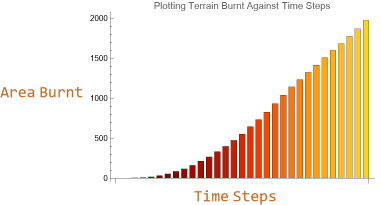
Plotting Terrain Area Burnt Against Time Steps
Plotting Terrain Area Burnt Against Time Steps
We created a visualization to plot the area burnt against time steps . This would be particularly beneficial for fire mitigation strategies because we can model the progression of the fire overtime .
In[]:=
timeSeriesPlot[]:=Module[{frames,history,listOfBurnt},frames=runFireSimulation[];history=frames["FireHistory"];listOfBurnt=Table[countBurned[history[[i]]],{i,Length[history]}];Labeled[BarChart[listOfBurnt,ColorFunction->"SolarColors",ChartStyle->"SolarColors",PlotLabel->"Plotting Terrain Burnt Against Time Steps"],{"Time Steps","Area Burnt"},{Bottom,Left}]]
04. Modeling 3D Wildfire Spread
04. Modeling 3D Wildfire Spread
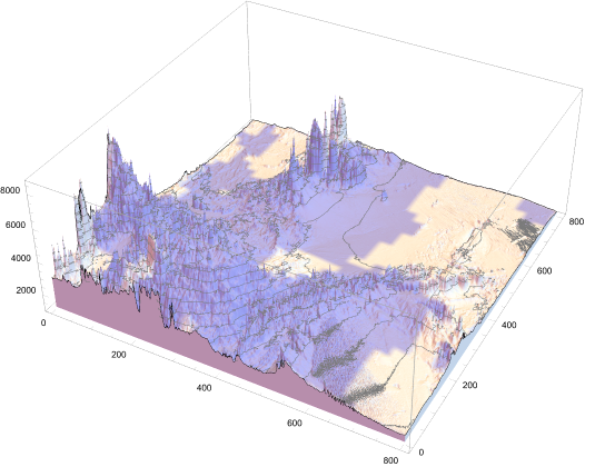
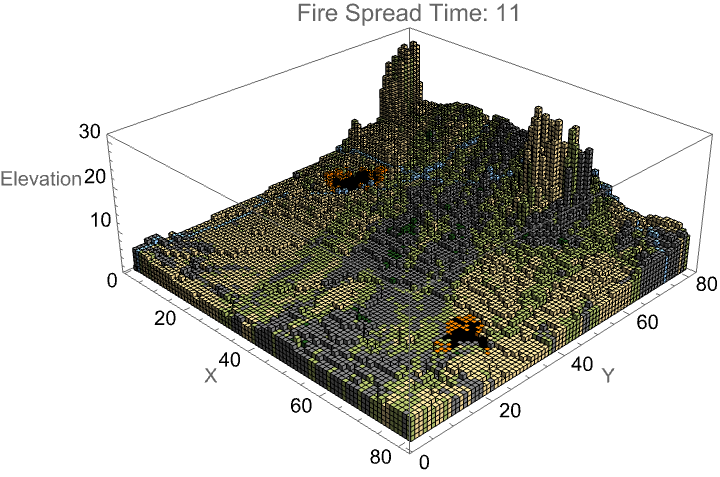
This section aims to extend our 2D fire spread framework into a 3D simulation. Three-dimensional visualization helps us understand how topography influences fire spread. By combining elevation data with satellite imagery, we create realistic landscape representations that clearly show why fires follow certain paths.
Creating 3D Terrain
Creating 3D Terrain
We implement the create3DTerrainArray function to create a terrain that accurately reflects a geographic location’s elevation.
create3DTerrainArray converts two flat datasets—elevation and land cover—into a volumetric “voxel” block, which helps to run the simulation in 3D. First it measures the smallest and largest elevations in the selected region, then linearly rescales every height so that the lowest point maps to layer 1 and the summit reaches the user-defined maxHeight. It allocates a cube of zeros whose vertical dimension equals this height budget and whose horizontal dimensions match the grid size. The routine then steps over every cell (i, j), looks up its rescaled height, and copies the terrain code for that surface patch into every voxel from the ground layer up to that height. The result is a stacked integer array in which empty space is 0, water, grass, forest and other patch types occupy realistic columns, and the top layer traces the true relief of the landscape.
In[]:=
create3DTerrainArray[elevationGrid_,terrainGrid_,gridSize_,maxHeight_:50]:=Module[{array3D,scaledElevation,minElev,maxElev,height},minElev=Min[elevationGrid];maxElev=Max[elevationGrid];scaledElevation=Rescale[elevationGrid,{minElev,maxElev},{1,maxHeight}];array3D=ConstantArray[0,{maxHeight,gridSize,gridSize}];Table[height=Round[scaledElevation[[i,j]]];Table[array3D[[h,i,j]]=terrainGrid[[i,j]],{h,1,height}],{i,gridSize},{j,gridSize}];array3D]
This preprocessing stage is crucial because the fire model can now be rendered in three dimensions without expensive geometry calculations at every time step.
Mapping Fire State to 3D Terrain
Mapping Fire State to 3D Terrain
The mapFireTo3D function maps the 2D fire grid onto a 3D array.
This function projects a two-dimensional fire state onto the voxel terrain built earlier. After rescaling the elevation grid to the voxel range, the routine locates the surface layer for every horizontal cell (i, j). At that layer it writes a code that represents the fire condition, values 11–20 for the ten burning stages, 25 for ash, leaving all lower voxels unchanged. The result, fireArray3D, is the original terrain array with its visible surface recolored to reflect the current fire front.
In[]:=
mapFireTo3D[array3D_,fireGrid_,terrainGrid_,elevationGrid_,maxHeight_:50]:=Module[{fireArray3D=array3D,scaledElevation,minElev,maxElev,height,fireState},minElev=Min[elevationGrid];maxElev=Max[elevationGrid];scaledElevation=Rescale[elevationGrid,{minElev,maxElev},{1,maxHeight}];Table[height=Round[scaledElevation[[i,j]]];fireState=fireGrid[[i,j]];If[fireState>0,Which[fireState<=10,fireArray3D[[height,i,j]]=10+fireState,fireState==11,fireArray3D[[height,i,j]]=25]],{i,Length[fireGrid]},{j,Length[fireGrid[[1]]]}];fireArray3D]
This mapping step isolates visualisation from computation. The spread model remains in 2D, ensuring numerical efficiency, while the 3D overlay supplies an immediate spatial context that reveals how flames advance across slopes.
Visualizing 3D Fire Spread
Visualizing 3D Fire Spread
visualize3DFire renders the voxel cube returned by the mapping routine as a 3D scene. It first defines colorFunction, a fixed legend that turns the integer codes in the cube into terrain hues and fire hues: grass, sand, rock, forest, soil, water, ten orange burn stages, and black ash. It then scans every voxel position; wherever the stored value is non-zero it couples the appropriate colour with a unit Cuboid, assembling these coloured blocks in voxelData. A single call to Graphics3D flattens this list and returns the result.
In[]:=
visualize3DFire[array3D_,timeLabel_:""]:=Module[{voxelData,colorFunction},colorFunction=Which[#==0,Nothing,#==1,RGBColor[0.66,0.72,0.4],#==2,RGBColor[0.93,0.83,0.58],#==3,Gray,#==4,RGBColor[0.15,0.37,0.13],#==5,RGBColor[0.43,0.22,0.2],#==6,RGBColor[0.6,0.807843137254902,1.0],11<=#<=20,Orange,#==25,Black,True,Gray]&;voxelData=Table[If[array3D[[k,i,j]]!=0,{colorFunction[array3D[[k,i,j]]],Cuboid[{i,j,k}]},Nothing],{k,Length[array3D]},{i,Length[array3D[[1]]]},{j,Length[array3D[[1,1]]]}];Graphics3D[Flatten[voxelData],Axes->True,AxesLabel->{"X","Y","Elevation"},PlotLabel->"Fire Spread "<>timeLabel,ViewPoint->{2,-2,1.5},Lighting->"Neutral",ImageSize->Large]]
visualize3DFireSurface produces a shaded-relief map that drapes the current fire state over the true topography. It first collapses the separate terrain and fire matrices into a single displayGrid, translating each burning cell into an intensity code (11–20) and each burnt cell into 25 while passing through the underlying terrain codes elsewhere. It then builds a colorFunction that, for any rendered surface point, back-projects its x-y coordinates to the nearest grid cell, retrieves the corresponding code from displayGrid, and returns the appropriate hue. Finally, ListPlot3D draws the elevation lattice with color lookup, suppresses mesh lines, fixes the scale, labels axes, and tags the frame with an optional time stamp.
In[]:=
visualize3DFireSurface[elevationGrid_,fireGrid_,terrainGrid_,timeLabel_:""]:=Module[{displayGrid,colorFunction},displayGrid=Table[Which[fireGrid[[i,j]]>0&&fireGrid[[i,j]]<=10,10+fireGrid[[i,j]],fireGrid[[i,j]]==11,25,True,terrainGrid[[i,j]]],{i,Length[fireGrid]},{j,Length[fireGrid[[1]]]}];colorFunction=Function[{x,y,z},Module[{gridX=Round[x],gridY=Round[y],value},gridX=Clip[gridX,{1,Length[displayGrid]}];gridY=Clip[gridY,{1,Length[displayGrid[[1]]]}];value=displayGrid[[gridY,gridX]];Which[value==1,RGBColor[0.66,0.72,0.4],value==2,RGBColor[0.93,0.83,0.58],value==3,Gray,value==4,RGBColor[0.15,0.37,0.13],value==5,RGBColor[0.43,0.22,0.2],value==6,RGBColor[0.6,0.807843137254902,1.0],11<=value<=20,Blend[{Orange,Red},(value-11)/9],value==25,Black,True,Gray]]];ListPlot3D[elevationGrid,ColorFunction->colorFunction,ColorFunctionScaling->False,Mesh->None,PlotLabel->"Fire Spread on Terrain "<>timeLabel,AxesLabel->{"X","Y","Elevation"},ViewPoint->{2,-2,1.5},PlotRange->All,ImageSize->Large]]
2D Satellite Mapping Onto 3D Model
2D Satellite Mapping Onto 3D Model
The satelliteImagery function creates a 3D terrain visualization by combining satellite imagery with elevation data for a specified geographic location. It first retrieves a satellite image of the area (with range determined by the grid size), then processes a second image to highlight water features by recoloring them in blue with transparency. After compositing these images together, it fetches real elevation data from the same geographic region and creates a 3D surface plot where the combined satellite imagery is draped over the terrain as a texture. The result is a realistic 3D landscape visualization showing the actual topography with satellite imagery overlay, making water bodies visually distinct from the surrounding terrain.
In[]:=
satelliteImagery[gridSize_,location_]:=Module[{satelliteImage,range,riverImage,fullSatelliteImage},range=gridSize*0.1;satelliteImage=GeoImage[GeoPosition[location],GeoRange->range];riverImage=Rasterize[ImageRecolor[Binarize[ColorNegate[GeoImage[location,GeoRange->range]]],{White->RGBColor[0,0,Rational[2,3],0.5],Black->RGBColor[0.5,0.5,0.5,0]}]];fullSatelliteImage=ImageCompose[satelliteImage,riverImage];ListPlot3D[QuantityMagnitude[GeoElevationData[GeoRange->{GeoPosition[location-{range,range}/2],GeoPosition[location+{range,range}/2]}]],MeshFunctions{#3&},PlotRange->All,PlotStyle->Texture[ImageRotate[fullSatelliteImage,3Pi/2]],Filling->Bottom,FillingStyleOpacity[1],ImageSize->1000]]
Generating 3D Terrain
Generating 3D Terrain
This generate3DTerrain function generates a 3D terrain visualization where both elevation and terrain type are displayed together. It first calls mapTerrainValues to get a 3D array containing height values and terrain type codes for each grid position. The function then creates a 3D surface plot using ListPlot3D where the surface height comes from the height array, but the coloring is determined by looking up each position’s terrain type in a global $terrainLookup table. This allows the visualization to show topographical features while simultaneously indicating what type of terrain exists at each location through color-coding, creating a comprehensive landscape representation.
In[]:=
generate3DTerrain[gridSize_,location_]:=Module{mappedTerrain,heightArray,terrainTypeArray,threeDPlot},mappedTerrain=mapTerrainValues[gridSize];heightArray=mappedTerrain[[All,All,1]];terrainTypeArray=mappedTerrain[[All,All,2]]; threeDPlot= ListPlot3DheightArray,ColorFunction->Function[{x,y,z},$terrainLookup[terrainTypeArray[[Round[y],Round[x]]]]],ColorFunctionScaling->False,Mesh->None
The run3DFireSimulation mirrors the functions of runFireSimulation in 3D rather than 2D. Both (1) acquire or generate matching terrain, elevation, and empty-fire grids; (2) open an interactive dialog so the user can place ignition points while preventing water-cell selection; (3) seed those points with vegetation-specific burn times; (4) drive a time-stepped loop that repeatedly invokes the core spread rule to update the fire state; and (5) assemble a set of visual outputs plus the complete fire-history tensor for later analysis. The main difference is that the 3D version adds one transformation and one extra view: it converts the terrain into a voxel stack and, after each spread step, maps the current fire grid into that volume for full volumetric rendering alongside the familiar surface plot.
run3DFireSimulation[gridSize_:40,initialFires_:2,timeSteps_:20,ignitionProbability_:0.8,windSpeed_:0.3,windDirection_:{1,0},moisture_:0.2,uphillMultiplier_:1.5,downhillMultiplier_:0.7,location_:Automatic,maxHeight_:30]:=Module[{terrainAndElev,terrainGrid,elevationGrid,fireGrid,actualLocation,firePoints,result,fireHistory,array3D,animation3D,animationSurface,gridPos,terrain,props,fire3D},actualLocation=If[location===Automatic,getRandomEarthLocation[],location];terrainAndElev=initializeTerrainGrid[gridSize,actualLocation];terrainGrid=terrainAndElev[[1]];elevationGrid=terrainAndElev[[2]];fireGrid=ConstantArray[0,{gridSize,gridSize}];array3D=create3DTerrainArray[elevationGrid,terrainGrid,gridSize,maxHeight];result=DialogInput[DynamicModule[{currentPoint={15,15},selectedPoints={}},Column[{Text["Click on the terrain to place fire starting points"],Text[Dynamic["Points selected: "<>ToString[Length[selectedPoints]]<>"/"<>ToString[initialFires]]],LocatorPane[Dynamic[currentPoint],plotTerrain[terrainGrid,"Select Fire Starting Points"],Appearance->Graphics[{Red,PointSize[0.05],Point[{0,0}]}]],Row[{Button["Add Fire Point",gridPos={Clip[Round[currentPoint[[2]]],{1,gridSize}],Clip[Round[currentPoint[[1]]],{1,gridSize}]};If[terrainGrid[[gridPos[[1]],gridPos[[2]]]]!=6,AppendTo[selectedPoints,gridPos],MessageDialog["Cannot place fire on water!"]],Enabled->Dynamic[Length[selectedPoints]<initialFires]],Button["Reset",selectedPoints={}],Button["Run Simulation",If[Length[selectedPoints]>0,DialogReturn[selectedPoints],MessageDialog["Please select at least one fire point!"]],Enabled->Dynamic[Length[selectedPoints]>0]],Button["Cancel",DialogReturn[$Canceled]]}]}]]];If[result===$Canceled,Return[$Canceled]];firePoints=result;Table[terrain=terrainGrid[[pos[[1]],pos[[2]]]];props=getPatchProperties[terrain];fireGrid[[pos[[1]],pos[[2]]]]=props["burnTime"];,{pos,firePoints}];fireHistory=NestList[fireSpreadRule[terrainGrid,#,elevationGrid,gridSize,ignitionProbability,windSpeed,windDirection,moisture,uphillMultiplier,downhillMultiplier]&,fireGrid,timeSteps];animation3D=Table[fire3D=mapFireTo3D[array3D,fireHistory[[t]],terrainGrid,elevationGrid,maxHeight];visualize3DFire[fire3D,"Time: "<>ToString[t-1]],{t,Length[fireHistory]}];animationSurface=Table[visualize3DFireSurface[elevationGrid,fireHistory[[t]],terrainGrid,"Time: "<>ToString[t-1]],{t,Length[fireHistory]}];<|"VoxelAnimation"->ListAnimate[animation3D,AnimationRunning->True,AnimationRate->1],"FireHistory"->fireHistory,"TerrainGrid"->terrainGrid,"ElevationGrid"->elevationGrid,"Location"->actualLocation,"FinalVoxelPlot"->Last[animation3D],"FinalSurfacePlot"->Last[animationSurface]|>]
05. Optimizing Fire Suppressant Placement
05. Optimizing Fire Suppressant Placement
Now that we have created a wildfire simulation, we create a risk prediction algorithm to identify the optimal areas to place fire suppressant.
Identify High Risk Areas
Identify High Risk Areas
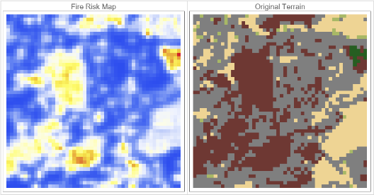
The predictFireSpread synthesizes terrain type, topography, wind, and moisture to yield a heat map of fire risks, which highlights where flames are most likely to advance over the next few time steps.
This function first allocates a zero-filled risk grid. For each cell that is not water (code 6) or already burned ground (code 3), it assigns a basal susceptibility that is inversely proportional to the patch’s flammability rating obtained from getPatchProperties. This baseline is reduced as overall fuel moisture rises and is amplified by wind strength. The algorithm then blends the cell’s value with the average risk of its eight neighbors, smoothing local extremes and reflecting contagious spread. Next, it adds a directional wind bonus: for each neighbor that lies broadly down-wind (alignment > 0.5), the risk is incremented in proportion to both wind speed and directional alignment. Finally, it scales the risk by slope: cells upslope of a neighbor gain intensity because rising flames accelerate uphill, whereas downslope propagation is damped. After all cells are processed, the map is globally rescaled to the unit interval, a mild non-linear exponent (1.5) accentuates high-risk zones, and a Gaussian blur produces a continuous surface.
In[]:=
predictFireSpread[terrainGrid_,elevationGrid_,windSpeed_,windDirection_,moisture_,gridSize_,predictionSteps_:10]:=Module[{riskMap,patchProps,windFactor,moistureFactor,slopeFactor,neighbors,avgRisk,windAlignment},riskMap=Table[0.0,{gridSize},{gridSize}];Table[If[terrainGrid[[i,j]]==6||terrainGrid[[i,j]]==3,riskMap[[i,j]]=0,patchProps=getPatchProperties[terrainGrid[[i,j]]];riskMap[[i,j]]=(7-patchProps["flammability"])/6.0;moistureFactor=1-moisture;riskMap[[i,j]]*=moistureFactor;windFactor=1+windSpeed*2;neighbors=Select[{{i-1,j-1},{i-1,j},{i-1,j+1},{i,j-1},{i,j+1},{i+1,j-1},{i+1,j},{i+1,j+1}},1<=#[[1]]<=gridSize&&1<=#[[2]]<=gridSize&];avgRisk=Mean[Table[If[terrainGrid[[n[[1]],n[[2]]]]==6||terrainGrid[[n[[1]],n[[2]]]]==3,0,(7-getPatchProperties[terrainGrid[[n[[1]],n[[2]]]]][["flammability"]])/6.0],{n,neighbors}]];riskMap[[i,j]]=0.7*riskMap[[i,j]]+0.3*avgRisk;Table[windAlignment=windDirection.Normalize[{n[[1]]-i,n[[2]]-j}];If[windAlignment>0.5,riskMap[[i,j]]+=0.2*windSpeed*windAlignment],{n,neighbors}];Table[slopeFactor=(elevationGrid[[n[[1]],n[[2]]]]-elevationGrid[[i,j]]);If[slopeFactor>0,riskMap[[i,j]]*=(1+0.3*Tanh[slopeFactor*10]),riskMap[[i,j]]*=(1-0.2*Tanh[Abs[slopeFactor]*10])],{n,neighbors}];],{i,gridSize},{j,gridSize}];riskMap=Rescale[riskMap,{0,Max[riskMap]},{0,1}];riskMap=riskMap^1.5;GaussianFilter[riskMap,2]]
Applying a Controlled Burn Strategy
Applying a Controlled Burn Strategy
The applyControlledBurnStrategy function calls predictFireSpread to obtain a continuous danger surface (riskMap) that ranks every grid cell by its likelihood of ignition given the current wind, fuel moisture, and slope. If visual output is requested, the routine then presents a two-panel display: on the left, an ArrayPlot of the risk map rendered with Mathematica’s TemperatureMap palette so the hottest colours mark the most threatened corridors; on the right, the original terrain grid coloured with the project-wide $terrainColorRules. The side-by-side layout allows a manager to compare latent risk against vegetation types at a glance and decide where fire retardant should be placed.
In[]:=
applyControlledBurnStrategy[terrainGrid_,elevationGrid_,windSpeed_,windDirection_,moisture_,gridSize_,showVisualization_:True]:=Module[{riskMap,burnPatches,corridorBreaks,modifiedTerrain,allBurnCells,patchBurnArea,corridorBurnArea},riskMap=predictFireSpread[terrainGrid,elevationGrid,windSpeed,windDirection,moisture,gridSize];If[showVisualization,Grid[{{ArrayPlot[riskMap,ColorFunction->"TemperatureMap",PlotLabel->"Fire Risk Map",ImageSize->300],ArrayPlot[terrainGrid,ColorRules->$terrainColorRules,PlotLabel->"Original Terrain",ImageSize->300]}},Frame->All,FrameStyle->LightGray]]]
Running the Fire Suppressant Strategy
Running the Fire Suppressant Strategy
The visualizeRisks function provides a one-command way to generate a fire-risk map for any randomly selected landscape patch. This function first draws an arbitrary land location (getRandomEarthLocation), then invokes initializeTerrainGrid, which downloads satellite imagery and elevation data for a square region whose side length is gridSize, returning two aligned arrays: vegetation type (terrainGrid) and topography (elevationGrid). With those layers in hand, it calls applyControlledBurnStrategy, passing through the governing environmental parameters so that function can (1) compute a probabilistic ignition surface via predictFireSpread, (2) overlay that risk on the terrain, and (3) display the side-by-side plots that support strategic fuel-treatment planning.
visualizeRisks[gridSize_:50,windSpeed_:0,windDirection_:{0,0},moisture_:0]:=Module[{location,terrainAndElev,terrainGrid,elevationGrid},location=getRandomEarthLocation[];terrainAndElev=initializeTerrainGrid[50,location];terrainGrid=terrainAndElev[[1]];elevationGrid=terrainAndElev[[2]];applyControlledBurnStrategy[terrainGrid,elevationGrid,windSpeed,windDirection,moisture,gridSize]]
06. Conclusion
06. Conclusion
As we see an increasing number of individuals at risk of being affected by wildfires, it is critical that we work to address this threat computationally. To accomplish that, we developed a cellular-automaton model that fuses satellite-derived land-cover maps with elevation data and simulates fire behaviour under varying wind, slope, moisture, radiant-heat, and ember-lofting conditions. Then building on these simulations, we introduced an optimisation routine that pinpoints the most vulnerable cells to direct fire retardant placement.
07. Future Direction
07. Future Direction
In the future, we would like to calibrate our simulation to real-world fire-spread data, aligning cellular-automaton parameters with observed ignition sequences, burn perimeters, and rate-of-spread measurements. Once those dynamics are tuned, we plan to refine the terrain layer by adding a richer catalogue of patch types such as residential blocks, industrial sites, croplands, and distinct vegetation classes so the model can capture wildland-urban-interface scenarios more effectively. On the optimisation side, we hope to implement a framework that applies gradient-descent or related solvers to locate globally efficient retardant corridors. Finally, we will embed operational considerations such as aircraft travel time, crew mobilisation delays, and refill cycles into the cost function in order to ensure that recommended strategies are optimal and feasible.
Acknowledgements
Acknowledgements
I would first like to extend a thank you to the Wolfram High School Summer Research Program team and Stephen Wolfram for giving me the opportunity to work on this project. Next I want to thank my mentor, Anton Antonov, who gave me immense amounts of support throughout my project. And to Ethan Kong and William Choi-Kim and all the other TAs and directors, thank you so much for the all the technical advice and help you’ve given me. yodahh67
References
References
[XL1] Li, Xingdong, et al. “Simulating Forest Fire Spread with Cellular Automation Driven by a LSTM Based Speed Model.” Fire, vol. 5, no. 1, Multidisciplinary Digital Publishing Institute, Jan. 2022, pp. 13–13, https://doi.org/10.3390/fire5010013. Accessed 7 July 2025.
[RR1] Rothermel, Richard C. 1972. A mathematical model for predicting fire spread in wildland fuels. Res. Pap. INT-115. Ogden, UT: U.S. Department of Agriculture, Intermountain Forest and Range Experiment Station. 40 p.
[WRC1] “Homepage - Wildfire Risk to Communities.” Wildfire Risk to Communities, 8 May 2025, wildfirerisk.org/. Accessed 10 July 2025.
[GC1] Morphological Analysis of River Tributaries and Flood Plains: A Multi-Dimensional Approach by George Cheng Wolfram Community, STAFF PICKS, July 13, 2023
https://community.wolfram.com/groups/-/m/t/2964526
https://community.wolfram.com/groups/-/m/t/2964526
CITE THIS NOTEBOOK
CITE THIS NOTEBOOK
Modeling 3D fire spread using cellular automata and optimizing fire suppressant placement
by Kelly Liu
Wolfram Community, STAFF PICKS, July 10, 2025
https://community.wolfram.com/groups/-/m/t/3502932
by Kelly Liu
Wolfram Community, STAFF PICKS, July 10, 2025
https://community.wolfram.com/groups/-/m/t/3502932