ORIGINAL BOOK: Trifce Sandev, Alexander Iomin (2022), Special Functions of Fractional Calculus: Applications to Diffusion and Random Search Processes, World Scientific Publishing Company, ISBN: 9789811252969. DOI: https://doi.org/10.1142/12743
AMAZON: https://a.co/d/0S5WVcx
KOBO: https://www.kobo.com/ww/en/ebook/special-functions-of-fractional-calculus
AMAZON: https://a.co/d/0S5WVcx
KOBO: https://www.kobo.com/ww/en/ebook/special-functions-of-fractional-calculus
This book addresses technical issues comprising the concept of special functions of anomalous transport with applications to fractional kinetics. An overview of special functions, such as the Fox H-function and the Mittag-Leffler functions is provided together with fractional calculus and their applications in diffusion and random search processes are discussed in detail. Detailed calculations of various examples of anomalous diffusion, random search and stochastic resetting processes are presented in such a way that the reader can easily follow the analysis. The implementation of Wolfram Mathematica is demonstrated, as well. The book is intended for advanced undergraduate and graduate students and researchers in physics, mathematics and other natural sciences due to the various examples provided in the book.
Contents:
Contents:
1 Mathematical Background2 Fox H-Function and Related Functions3 Elements of Random Walk Theory4 CTRW on Combs5 Heterogeneous Diffusion Processes6 Diffusion Processes with Stochastic Resetting7 Random Search8 Diffusion on Fractal Tartan9 Finite-Velocity Diffusion10 Appendices: A Functional Calculus B Stochastic Differential Equations C Large Deviation Principle D Fractals and Fractal Dimension E Implementation of Wolfram Mathematica
Special attention throughout the book is devoted to the way how Wolfram Language is applied to perform integral transforms, for evaluation of various special functions, with special attention to evaluations and calculations of the Mittag-Leffler functions and the Fox H-functions.
In an appendix of the book some functions and transforms, which are implemented in Wolfram Mathematica and used in the main text of the book are described. NumericalInversion.m package from Wolfram Mathematica is employed, where the inverse Laplace and Fourier transform techniques by Durbin, Stehfest, Weeks, Piessens, and Crump are used. Below, two examples of these calculations from the appendix are suggested.
In an appendix of the book some functions and transforms, which are implemented in Wolfram Mathematica and used in the main text of the book are described. NumericalInversion.m package from Wolfram Mathematica is employed, where the inverse Laplace and Fourier transform techniques by Durbin, Stehfest, Weeks, Piessens, and Crump are used. Below, two examples of these calculations from the appendix are suggested.
One parameter Mittag-Leffler function: (https://reference.wolfram.com/language/ref/MittagLefflerE.html)
The one parameter Mittag-Leffler function is defined by
E
α
∞
∑
k=0
k
z
Γ(αk+1)
where z ∈ C, Re(α)>0 and Γ(z) is the gamma function.
It is a generalization, for example, of the exponential function
It is a generalization, for example, of the exponential function
E
1
∞
∑
k=0
k
(±z)
Γ(k+1)
∞
∑
k=0
k
(±z)
k!
±z
e
as well as, trigonometric and and hyperbolic functions
E
2
2
z
∞
∑
k=0
k
(-1)
2k
z
Γ(2k+1)
∞
∑
k=0
k
(-1)
2k
z
(2k)!
E
2
2
z
∞
∑
k=0
2k
z
Γ(2k+1)
∞
∑
k=0
2k
z
(2k)!
One of the most important class of functions in the theory of fractional differential equations is the associated one parameter Mittag-Leffler function
ℰ
α
E
α
α
t
Its Laplace transform reads
L[(t;∓λ)]=L[(∓)]=∓λ,Re(s)>.
ℰ
α
E
α
α
λt
α-1
s
α
s
1/α
(|λ|)
The one parameter Mittag-Leffler function is implemented in the Wolfram Language as MittagLefflerE[α, z].
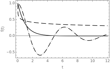
Example: We will use the Durbin technique of the inverse Laplace transform of
F(s)=+λ,λ>0,
α-1
s
α
s
which is the Laplace image of the associated one parameter Mittag-Leffler function,
f(t)=
E
α
α
t
to plot the associated one parameter Mittag-Leffler function. The same plot can be reproduced by MittagLefflerE[α, z].
Plot with numerical inverse Laplace transform
Plot with numerical inverse Laplace transform
In[]:=
Clear["Global`*"]<<NumericalInversion.mF[α_,λ_,s_]:=+λ;f[α_,λ_,t_]:=Piessens[F[α,λ,s],s,t];
α-1
s
α
s
In[]:=
Plot[{f[1/4,1,t],f[1,1,t],f[7/4,1,t]},{t,0,12},PlotRange->All,FrameTrue,FrameLabel{"t","f(t)"},FrameStyle(FontFamily"Helvetica"),LabelStyle(FontSize12),PlotStyle{{Black,Dashing[{Large,Medium}]},Black,{Black,Dashing[{0,Small,Large,Small}]}}]
Out[]=

Graphical representation of the one parameter Mittag-Leffler function for and (dashed line), (exponential function – solid line), and (dot-dashed line).
λ=1
α=1/4
α=1
α=7/4
Plot with MittagLefflerE[α, z]
In[]:=
Clear["Global`*"]
In[]:=
PlotMittagLefflerE14,-,Exp[-t],MittagLefflerE74,-,{t,0,12},PlotRange->All,FrameTrue,FrameLabel{"t","f(t)"},FrameStyle(FontFamily"Helvetica"),LabelStyle(FontSize12),PlotStyle{{Black,Dashing[{Large,Medium}]},Black,{Black,Dashing[{0,Small,Large,Small}]}}
1/4
t
7/4
t
Out[]=
The Fox H-function is a very general function. For example, the Mittag-Leffler function is a special case of the Fox H-function. However there are also many other well known special functions like Bessel functions, can be expressed by means of the Fox H-functions. Here we demonstrate the application of Wolfram Mathematica as a solution of a fractional diffusion equation. The Fox H-function is implemented in the Wolfram Language as followsFoxH[ {{{, }, . . . , {, }}, {{, }, . . . , {, }}},{{{, }, . . . , {, }}, {{, }, . . . , {, }}}, z ].
a
1
A
1
a
n
A
n
a
n+1
A
n+1
a
p
A
p
b
1
B
1
b
m
B
m
b
m+1
B
m+1
b
q
B
q
Example: In Wolfram Mathematica, the numerical inverse Laplace transform can be implemented together with the numerical inverse Fourier transform. We demonstrate the Stehfest technique of the inverse Fourier-Laplace transform of
p(k,s)=+D,λ>0,
α-1
s
α
s
β
(k|)
which is the solution of the space-time fractional diffusion equation in Fourier-Laplace space. The inverse Fourier-Laplace transform of it yields the Fox H-function, i.e.,
P(x,t)=H
.
1
β|x|
|x|
1/β
(D)
α
t
(1,1/β) | (1,α/β) | (1,1/2) |
(1,1) | (1,1/β) | (1,1/2) |
We note that, when one performs the numerical inverse Fourier transform, one should multiply the expression by a factor 1/(2π)1/2 due to the different definition of the inverse Fourier transform in Mathematica.
Plot with numerical inverse Fourier-Laplace transform
Plot with numerical inverse Fourier-Laplace transform
In[]:=
Clear["Global`*"]<<NumericalInversion.mF[α_,β_,d_,s_,w_]:=s^(α-1)/(s^α+dAbs[w]^β);f[α_,β_,d_,t_,x_]:=1/(2Pi)^(1/2)NFourierStehfest[F[α,β,d,s,w],{s,w},{t,x}];
In[]:=
Plot[{f[0.5,2,1,1,x],f[0.25,1.75,1,1,x],f[1,1.5,1,1,x]},{x,-5,5},PlotRange->All,FrameTrue,FrameLabel{"x","P(x,t)"},FrameStyle(FontFamily"Helvetica"),LabelStyle(FontSize12),PlotStyle{Black,{Black,Dashing[{Large,Medium}]},{Black,Dashing[{0,Small,Large,Small}]}}]
Out[]=
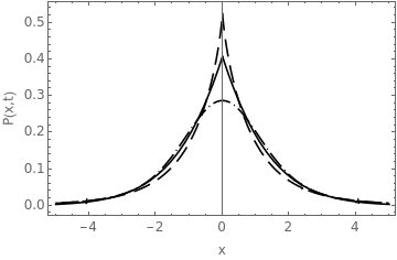
Graphical representation of (E.15) for , and , (solid line), , (dashed line), , (dot-dashed line).
t=1
D=1
α=0.5
β=2
α=0.25
β=1.75
α=1
β=1.5
CITE THIS NOTEBOOK
CITE THIS NOTEBOOK
Special Functions of Fractional Calculus: Applications to Diffusion and Random Search Processes
by Trifce Sandev and Alexander Iomin
Wolfram Community, STAFF PICKS, November 29, 2023
https://community.wolfram.com/groups/-/m/t/3073954
by Trifce Sandev and Alexander Iomin
Wolfram Community, STAFF PICKS, November 29, 2023
https://community.wolfram.com/groups/-/m/t/3073954