CITE THIS NOTEBOOK: Tool for graphing images of transformations: trnsfrm by A Horwitz. Wolfram Community MAR 24 2023.
No advanced math here, just a tool which I use in the classroom and for personal entertainment. This notebook has demonstrations for using trnsfrm, a program which directly applies a transformation map to points within primitives Point, Line and Polygon in an existing Graphics or Grapics3D picture in order to draw its image in the range, either in 2 or 3 dimensions. I don’t remember the edition or page number, but the code for shape2 is similar to an example in Roman Maeder’s ”Programming in Mathematica”. I wrote trnsfrm for Version 3, but added code for Version 6 and higher to be able to transform points inside GraphicComplex lists . It’s usually fast and reliable, though not always perfect. I recently I had to add /.Indeterminate0 on the last command in order to make it draw a graph when there are error messages for an Indeterminate coordinate. If it fails to work because of errors in getting a PlotRange , or you want a plot range different from the default choice, you can list the option PlotRange->_ using a specific range or “All”. Sometimes the lighting of 3 dimensional images is odd: bright on one side and very dark on the other side.
To minimize notebook size , most 2 dimensional images are in bitmap format. The same is true for a few 3 dimensional images: these can't be rotated unless you execute commands to draw them again.
The Program
The Program
If your transformation is written as a vector with expressions in terms of x , y and z, then you must list {x,y,z} as an argument in trnsfrm. If your transformation is a vector function f[x,y] or f[x,y,z] , then you must list the variables . If your transformation has the form f[{x,y}] or f[{x,y,z}], then writing “f “ without listing the variables will work , unless f is defined as a pure function: then you will need to write f[x,y, z] and list {x,y,z} in the arguments .
trnsfrm[shape_,fexpression_,{x_,y_},opts___]:=Module[{xx,yy,g},g[{xx_,yy_}]:=fexpression/.{xxx,yyy};(*Print[g[{u,v}]]*)trnsfrm[shape,g,opts]];trnsfrm[shape_,fexpression_,{x_,y_,z_},opts___]:=Module[{xx,yy,zz,g},g[{xx_,yy_,zz_}]:=fexpression/.{xxx,yyy,zzz};(*Print[g[{u,v,w}]]*)trnsfrm[shape,g,opts]];trnsfrm[shape_,g_,opts___]:=Block[{plotshells,headlist,heads,gimage,mapg,choice,predim,postdim,shape2},plotshells={Join[{opts},Options[shape]],Join[{opts},Options[Graphics]],Join[{opts},Options[Graphics3D]]};headlist={Graphics,Graphics3D}; shape2=shape/.{poly:Polygon[_]Map[g[#1]&,poly,{2}],line:Line[_]Map[g[#1]&,line,{2}],point:Point[_]Map[g[#1]&,point,{1}],
grpcmplx:GraphicsComplex[_,u___]GraphicsComplex[Map[g[#]&,grpcmplx[[1]],{1}],u]
,arrow:Arrow[_]Map[g[#1]&,arrow,{2}]
}; mapg=Map[g[#]&,{{u,v},{u,v,w}}]; Print["the map is ",DeleteCases[mapg,g[___]][[1]]];predim=4-Position[mapg,g[_]]1,1;Print["dimension of the preimage = ",predim];postdim=Length[Flatten[DeleteCases[mapg,g[___]],1]];Print["dimension of the image = ",postdim]; If[predim/postdim===1,choice=1,choice=postdim];rplace[a_,b_,c_]:=a/.c->b;shape2=rplace[shape2,plotshells[[choice]],shape2〚2〛];heads=headlistpostdim-1;shape2=rplace[shape2,heads,shape2〚0〛];shape2/.Indeterminate0.];Here are transformations for mapping points in the plane into planar regions and onto parametric surfaces in space.
grph[g_][{x_,y_}]:={x,y,g[{x,y}]};ftorus[bigr_,smallr_][{x_,y_}]:=N[{(bigr+smallr*Cos[x])Cos[y],(bigr+smallr*Cos[x])Sin[y],smallr*Sin[x]}];fpolar[{r_,theta_}]:=N[{r*Cos[theta],r*Sin[theta]}];(*fcylinderandfspherecanbeusedformappingcylindricalandsphericaltorectangularcoordinates*)fcylinder[r_][{theta_,z_}]:=N[{r*Cos[theta],r*Sin[theta],z}];fsphere[ro_][{phi_,theta_}]:=N[{ro*Sin[phi]Cos[theta],ro*Sin[phi]Sin[theta],ro*Cos[phi]}];cone[slope_][{x_,y_}]:={x,y,slope*Sqrt[x^2+y^2]};conepolar[slope_][{r_,theta_}]:={r*Cos[theta],r*Sin[theta],slope*r};fellipsoid[a_,b_,c_][{phi_,theta_}]:=N[{a*Sin[phi]Cos[theta],b*Sin[phi]Sin[theta],c*Cos[phi]}];moebiusmap[{u_,t_}]:= N[{6*Cos[u]+t*Cos[u/2]*Cos[u],6*Sin[u]+t*Cos[u/2]*Sin[u],t*Sin[u/2]}];
These are for images of fractional linear transformations of z=x+Iy.
cmplxdiv[{x_,y_},{v_,w_}]:=(1/(v^2+w^2))*{x*v+y*w,v*y-x*w};fraclin[{a_,b_},{c_,d_}][{x_,y_}]:=cmplxdiv[{a*x+b,a*y},{c*x+d,c*y}];
Here is a composition of maps for drawing a "bumpy torus" parametric surface.
newtorus[bigr_,smallr_][{x_,y_,z_}]:=N[{(bigr+(smallr+z)*Cos[x])Cos[y],(bigr+(smallr+z)*Cos[x])Sin[y],(smallr+z)*Sin[x]}];g32:=(Cos[3*#[[2]]]*Sin[2*#[[1]]])&;bumpytorus[bigr_,smallr_][{x_,y_}]:=newtorus[bigr,smallr][{x,y,g32[{x,y}]}]
Coordinate Transformations
Coordinate Transformations
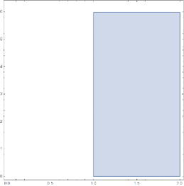
Here is how to use the conepolar map to draw a frustum. For the domain, PlotPoints40 is used to ensure the boundary circles don’t look like polygons. The second frustum uses plot options for axis labels and font size.
In[]:=
domain=RegionPlot[(1≤r≤2)&&(0≤theta≤1.9*Pi),{r,0,2},{theta,0,2*Pi},PlotPoints40]
Out[]=
(*transformationconepolar[slope]hasinputvariablesintheformofalist{r,theta},soinputvariablesneednotbeusedasargumentsintrnsfrm*)
In[]:=
conepolar[slope_][{r_,theta_}]:={r*Cos[theta],r*Sin[theta],slope*r};
In[]:=
trnsfrm[domain,conepolar[1]]
the map is {uCos[v],uSin[v],u}
dimension of the preimage = 2
dimension of the image = 3
Out[]=

Using conepolar[slope][{r, t}] requires using input variables {r,t}, in the arguments.
In[]:=
trnsfrm[domain,conepolar[5][{r,t}],{r,t},AxesTrue,AxesLabel{"x","y","z"},LabelStyle16]
the map is {uCos[v],uSin[v],5u}
dimension of the preimage = 2
dimension of the image = 3
Out[]=

We use fsphere to transform spherical to rectangular coordinates, in order to draw a spherical element of volume.
In[]:=
fsphere[ro_][{phi_,theta_}]:=N[{ro*Sin[phi]Cos[theta],ro*Sin[phi]Sin[theta],ro*Cos[phi]}];
inequalities:=(1≤ro≤1.2)&&(Pi/6≤phi≤1.2*Pi/6)&&(Pi/3≤theta≤1.2*Pi/3);smallvol=RegionPlot3D[inequalities//Evaluate,{ro,0,1.5},{phi,0,Pi/4},{theta,0,Pi/2},PlotPoints40,LabelStyle16,AxesLabel{"ρ","ϕ","θ"},MeshNone,ImageSize200];(*ThedefaultAxesLabelandBoxRatiosarethosefromdeltavolumesonewonesmustbespecifiedasplotoptions*)volelement=trnsfrm[smallvol,fsphere[ro][{phi,theta}],{ro,phi,theta},AxesLabel{"x","y","z"},BoxRatiosAutomatic,ImageSize300];{smallvol,volelement}//Row
the map is {uCos[w]Sin[v],uSin[v]Sin[w],uCos[v]}
dimension of the preimage = 3
dimension of the image = 3
Out[]=


Mapping Images on a Plane to Surfaces
Mapping Images on a Plane to Surfaces
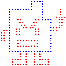
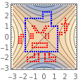
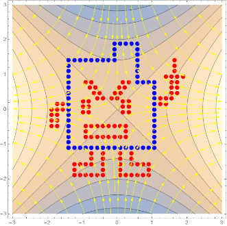
The following example uses a mooninite which fits inside a [-2.5, 2.5] x [-2.5, 2.5] square. These are its points.
redpoints=;bluepoints=;
In[]:=
mooninite=Graphics[{PointSize[.02],{Red,Map[Point,redpoints]},{Blue,Map[Point,bluepoints]}}]
Out[]=
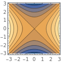
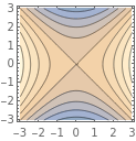
We draw level curves of . ContourPlot has no opacity settings, but we are able to make its graphs translucent by attaching an Opacity[.5] directive to each Polygon.
f(x,y)=-
2
x
2
y
In[]:=
contourpic=ContourPlot[x^2-y^2,{x,-3,3},{y,-3,3},PlotPoints75];contourlite=contourpic/.Polygon[x_]{Opacity[.5],Polygon[x]};{contourpic,contourlite}//Row
Out[]=
Wemapthemooninitetogetherwithlevelcurvesof f(x,y)=-toatopographicsaddlesurfacebygraphingf(x,y)roundedtothenextsmallesteveninteger
2
x
2
y
We map the mooninite together with level curves of to a topographic saddle surface by graphing f(x,y) rounded to the next smallest even integer.
f(x,y)=-
2
x
2
y
combined=Show[contourlite,mooninite,AspectRatioAutomatic];surface=trnsfrm[combined,{x,y,Round[x^2-y^2,2]},{x,y},BoxRatios{1,1,.7},AxesTrue,AxesLabel{"x","y","z"}];{combined,surface}//Row
the map is {u,v,Round[-,2]}
2
u
2
v
dimension of the preimage = 2
dimension of the image = 3
Out[]=

Shear Transformations
Shear Transformations
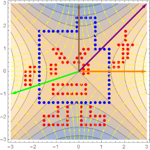
For showing a linear algebra class what vertical and horizontal shear transformations do, I’d like a domain with many features, for example adding vectors and flow lines to the combined picture above to make a new picture, combined1.
In[]:=
vec3={-3,-1};vec4={3,3};vec1={3,0};vec2={0,3};vectors=Graphics[{Thickness[.007],Orange,Arrow[{{0,0},vec1}],Brown,Arrow[{{0,0},vec2}],Green,Arrow[{{0,0},vec3}],Purple,Arrow[{{0,0},vec4}]},{AxesTrue,AxesLabel{"x","y","z"}}]/.Arrow[x_]->{Thickness[.01],Arrow[x]}
Out[]=

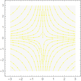
The flow lines are integral curves for the gradient field for f(x,y)=+. The curves are yellow against a light gray background.
2
x
2
y
vecfield=Grad[x^2-y^2,{x,y}];integcrvs=StreamPlot[vecfield,{x,-3,3},{y,-3,3},StreamStyleYellow,StreamPoints35,Epilog{Opacity[.21],LightGray,Polygon[{{-3,-3},{3,-3},{3,3},{-3,3}}]}]
Out[]=
In[]:=
combined1=Show[contourlite,mooninite,integcrvs,vectors,AspectRatioAutomatic]
Out[]=
In[]:=
{{combined1},{trnsfrm[combined1,{x,ax+y}/.a.5,{x,y},PlotRangeAll,PlotLabel"Vertical Shear"]},{trnsfrm[combined1,{x+ay,y}/.a.25,{x,y},PlotRangeAll,PlotLabel"Horizontal Shear",AxesTrue,AxesStyleDirective[Thickness[.01],Gray,Opacity[.5]],LabelStyle14]}}//TableForm
the map is {u,0.5u+v}
dimension of the preimage = 2
dimension of the image = 2
the map is {u+0.25v,v}
dimension of the preimage = 2
dimension of the image = 2
Out[]//TableForm=

Forbidden Planet
Forbidden Planet
We modify the pictures in combined1 by removing the vectors and multiplying points of the mooninite by .8 to reduce its size
In[]:=
newmoon=mooninite/.Point[x_]Point[.8*x];combined2=Show[contourlite,newmoon,integcrvs,AspectRatioAutomatic]
Out[]=
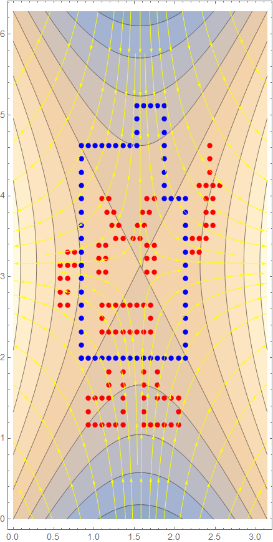
We reposition the domain to make it easy to map onto a sphere. The transformation maptonewdomain shifts the domain [-3, 3] x [-3, 3] to new rectangle [0, 6] x [0, 6], then multiplies by a factor of π/6 horizontally and π/3 vertically to make it into a rectangular region [0, π] x [0, 2π] ,
which will be mapped onto a sphere.
which will be mapped onto a sphere.
In[]:=
shift:=(#1+#2)&;shrink:=(#1*#2)&;maptonewdomain=shrink[shift[{x,y},{3,3}],{Pi/6,2*Pi/6}]
Out[]=
π(3+x),π(3+y)
1
6
1
3
We need PlotRangeAll because the default plot range does not show the entire image.
In[]:=
newdomain=trnsfrm[combined2,maptonewdomain,{x,y},PlotRangeAll]
the map is π(3+u),π(3+v)
1
6
1
3
dimension of the preimage = 2
dimension of the image = 2
Out[]=
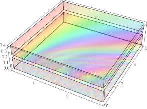
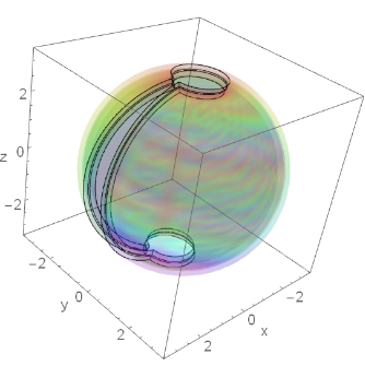
We draw a planet and an atmosphere, then show them together.
In[]:=
sfear=trnsfrm[newdomain,fsphere[3],AxesTrue,LabelStyle16,AxesLabel{"x","y","z"}]
the map is {3.Cos[v]Sin[u],3.Sin[u]Sin[v],3.Cos[u]}
dimension of the preimage = 2
dimension of the image = 3
Out[]=

In[]:=
layers=RegionPlot3D[(0.02≤z≤.2)||(.25≤z≤.4),{x,.085*Pi,.915*Pi},{y,0,1.9*Pi},{z,0,.4},ColorFunctionFunction[{x,y,z},Hue[(x)/(.01+y^2+z^2),1,1]],PlotStyleDirective[Red,Opacity[.12]],MeshFalse,BoxRatios{1,1,.3},PlotPoints50]
Out[]=
In[]:=
atmosfear=trnsfrm[layers,fsphere[z+3][{x,y}],{x,y,z},PlotRangeAll,BoxRatiosAutomatic,AxesTrue,AxesLabel{"x","y","z"},LabelStyle16]
the map is {(3.+w)Cos[v]Sin[u],(3.+w)Sin[u]Sin[v],(3.+w)Cos[u]}
dimension of the preimage = 3
dimension of the image = 3
Out[]=
In[]:=
planet=Show[sfear,atmosfear]
Out[]=

Roman Holiday
Roman Holiday
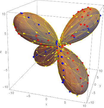
A link https://en.wikipedia.org/wiki/Roman_surface on Wikapedia describes a map f(x, y, z )=(yz, xz, xy) from a sphere onto a Roman surface. We use trnsfrm to find the f- image of sfear .
In[]:=
froman[x_,y_,z_]:={y*z,x*z,x*y};trnsfrm[sfear,froman[x,y,z],{x,y,z}]
the map is {vw,uw,uv}
dimension of the preimage = 3
dimension of the image = 3
In[]:=
romansurface= ;
;
Here’s what happens when you apply the Roman surface map f(x, y, z )=(yz, xz, xy) to a Roman surface. I typed “romansurface=” in front of the Roman surface graph, and shift-entered to assign the graphics to the name, then used it below. I won’t try to guess why it looks that way. A “bitmap” image is used to reduce file size.
In[]:=
trnsfrm[romansurface,froman[x,y,z],{x,y,z}]
the map is {vw,uw,uv}
dimension of the preimage = 3
dimension of the image = 3
Out[]=
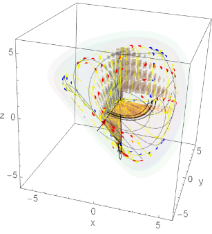
Using the Roman surface map f(x, y, z )=(yz, xz, xy) on the atmosphere yields a strange image which seems to be opaque rather than having Opacity[.12] as it did in the planet. Using f to transform the planet and atmosphere, or showing their separate images under f produces the same picture, which hides much of the Roman surface. A “ bitmap” image is used for the transformed planet with atmosphere.
In[]:=
trnsfrm[atmosfear,froman[x,y,z],{x,y,z}]
the map is {vw,uw,uv}
dimension of the preimage = 3
dimension of the image = 3
Out[]=

In[]:=
trnsfrm[planet,froman[x,y,z],{x,y,z}]
the map is {vw,uw,uv}
dimension of the preimage = 3
dimension of the image = 3
Out[]=