This essay was written as part of the Wolfram Emerging Leaders Program: Undergraduate, which is a year long, project-based program designed for gifted undergraduate students to take a deep dive into a topic of their choice. Students work remotely to take their project from ideation to completion, with the guidance of Wolfram experts. Wolfram Emerging Leaders Program participants are selected from the Wolfram High School Summer Research Program or the Wolfram Summer School, which is open to talented, STEM-oriented students.

Introduction

More than likely, you’ve heard of the popular joke “topologists can’t tell the difference between a coffee mug and a donut” at some point. Indeed, topologists seem to care quite a bit about holes. But maybe so should we. The theory of homology--the mathematical formalization of the notion of holes-- has proven to be a powerful tool in domains such as image processing, medical research, and machine learning, to name a few. We will dive into some of the fundamental concepts relevant to Topological Data Analysis, and show how they could be implemented in Mathematica. We will also take a detour into Discrete Morse Theory to explore how it could be used to build more efficient TDA algorithms.

Simplicial Homology

Betti numbers of abstract simplicial complexes

Geometric objects are often quite difficult to work with, especially in higher dimensions. The motivating philosophy of algebraic topology is therefore to study these objects indirectly through the lens of algebra. Homology theory, in particular, offers a way of associating the so-called homology groups with topological spaces, which encode certain global properties of the given space. The rank of the n-th homology group is known as the n-th Betti number, and for

n1,2

, these numbers could reasonably be interpreted as the number of n-dimensional holes in the space. In TDA settings, simplicial homology groups are of particular interest due to their combinatorial nature. These groups can be computed directly from an abstract simplicial complex, which is defined as a collection

S:

{

}

i,n

, where each

is some ordered set of points

[

,...,

]

, and for

k<n,

⊂

⇒

∈S

. That is to say, the faces of a simplex is also a member of the collection. To realize an abstract simplicial complex as a geometric one, we can imagine each

as a point in space, and

as the convex hull of such points. For instance:

In[]:=

S={{1},{2},{3},{4},{5},{1,5},{2,5},{1,3},{1,2},{2,3},{1,4},{2,4},{3,4},{1,2,3},{1,3,4},{1,2,4},{2,3,4}};HighlightMesh[MeshRegion[{{0,0,0},{1,0,0},{0,1,0},{0,0,1},{0,0,2}},{Line[{5,1}],Line[{5,2}],Tetrahedron[{1,2,3,4}]},MeshCellStyle->{{1,All}->Red}],Labeled[0,"Index"]]

Out[]=

Observing the geometric representation of S, we see that the hollow tetrahedron encloses a 2-dimensional hole, and there’s also a 1-dimensional hole (a loop) enclosed by {2,4,5}. This fact is captured by the rank of

and

, the 1st and 2nd simplicial homology groups of S. These groups are defined to be the quotient groups Ker

∂

n+1

, where

∂

(the k-th boundary operator) is the alternating formal sum

∂

[

,...,

]:

∑

i+1

(-1)



,..,



,..,



, with



denoting the omission of

to obtain a k-1 simplex. If we want to compute the rank of these groups, we could view

as a quotient vector space, whose dimension is then precisely the n-th Betti number. This gives us a simple way to compute the Betti numbers: write

∂

and

∂

n+1

as matrices, so that the n-th Betti number

is just Dim(Ker

∂

) - Rank(

∂

n+1

). The following is an implementation of this algorithm:

In[]:=

nSkeleton[complex_List,n_Integer]:=With[{A=Sort[#]&/@Cases[complex,x_/;Length[x]==n+1]//Sort},A[[#]]->SparseArray[{1,#}->1,{1,Length[A]}]&/@Range[1,Length[A]]]//AssociationboundaryVector[simplex_List,A_Association]:=(-1)^(#+1)*A[Drop[simplex,{#}]]&/@Range[1,Length[simplex]]//TotalboundaryOperator[complex_List,n_]:=With[{A=nSkeleton[complex,n-1],B=Sort[#]&/@Cases[complex,x_/;Length[x]==n+1]//Sort},If[n==0,{Array[0&,Length[B]]},Join[Sequence@@(boundaryVector[#,A]&/@B)]//Transpose]]BettiNumber[complex_List,n_Integer]:=With[{M1=boundaryOperator[complex,n],M2=boundaryOperator[complex,n+1]},If[M1=={},0,Dimensions[M1][[2]]-MatrixRank[M1]]-If[M2=={},0,MatrixRank[M2]]]

Testing this on S,

Print[BettiNumber[S,1]];Print[BettiNumber[S,2]]

As expected.

Graphs as simplicial complexes

Graphs are closely associated with simplicial structures. Give a graph G, we can define a simplicial complex

as follows:

[

,...,

]∈

if and only if

{

,...,

}

are spanned by a subgraph isomorphic to the complete graph

. This is only one of many ways to associate a simplicial structure with a graph; in fact, similar constructions can be made w.r.t. any monotone graph property (see [1]).

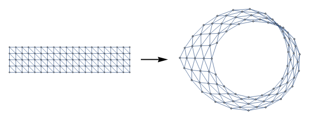
With this observation, an interesting application is that we can represent triangulations of various surfaces by ‘gluing together the boundaries of a diagonal grid graph with VertexContract[]. Below we construct a graph representing the Moebius strip (

≅Z

) by identifying two sides of a grid graph with reverse orientations:

diagonalGridGraph[n_,m_]:=UndirectedGraph[RelationGraph[ChessboardDistance[#1,#2]==1&&(#1[[1]]-#2[[1]]+#2[[2]]-#1[[2]])!=0&,GraphEmbedding@GridGraph[{n,m}]],VertexCoordinates->Join[Sequence@@Table[{i,j},{i,1,m},{j,1,n}]]]mobiusStripGrid[n_Integer,m_Integer]:=Graph[VertexContract[diagonalGridGraph[n,m],MobiusIdentifications[n,m]],VertexCoordinates->Automatic]MobiusIdentifications[n_,m_]:=N[{{1,#},{m,n+1-#}}&/@Range[1,n]]GraphicsRow[{diagonalGridGraph[5,20],Graphics[{Thick,{Arrowheads[Large],Arrow[{{0,0},{0.5,0}}]}}],mobiusStripGrid[5,20]}]

Out[]=

We could then compute the 0th and 1st Betti numbers from the simplicial complex associated with the cliques of the graph:

In[]:=

GraphComplex[g_Graph,n_]:=DeleteCases[Union[Sequence@@Subsets[#,n+2]&/@FindClique[g,Infinity,All]],{}]

In[]:=

GraphBettiNumber[g_Graph,n_]:=With[{K=GraphComplex[g,n]},BettiNumber[K,#]&/@Range[0,n]]GraphBettiNumber[mobiusStripGrid[5,20],1]

Out[]=

{1,1}

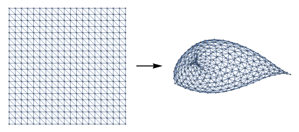
We could construct a real-projective plane (

≅

0

) by also identifying the horizontal sides in the same fashion:

In[]:=

RP2Identifications[n_,m_]:=Union[MobiusIdentifications[n,m],N[{{#,1},{m+1-#,n}}&/@Range[1,m]]]RP2Grid[n_Integer,m_Integer]:=Graph[VertexContract[diagonalGridGraph[n,m],RP2Identifications[n,m]],VertexCoordinates->Automatic]GraphicsRow[{diagonalGridGraph[20,20],Graphics[{Thick,{Arrowheads[Large],Arrow[{{0,0},{0.5,0}}]}}],RP2Grid[20,20]}]

Out[]=

Its oth through 2nd Betti numbers are:

In[]:=

GraphBettiNumber[RP2Grid[20,20],2]

Out[]=

{1,0,0}

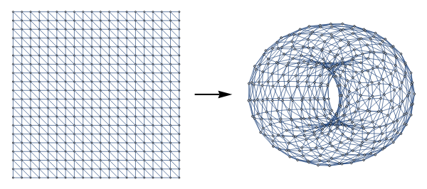
Or, we could have a Klein bottle (

≅Z⊕

0

) by identifying the horizontal edges in parallel orientation:

In[]:=

kleinBottleIdentifications[n_,m_]:=Join[MobiusIdentifications[n,m],N[{{#,1},{#,n}}&/@Range[1,m]]]kleinBottleGrid[n_Integer,m_Integer]:=Graph[VertexContract[diagonalGridGraph[n,m],kleinBottleIdentifications[n,m]],VertexCoordinates->Automatic]GraphicsRow[{diagonalGridGraph[20,20],Graphics[{Thick,{Arrowheads[Large],Arrow[{{0,0},{0.5,0}}]}}],kleinBottleGrid[20,20]}]

Out[]=

Where its oth through 2nd Betti numbers are:

GraphBettiNumber[kleinBottleGrid[20,20],2]

Out[]=

{1,1,0}

Topological data analysis

With the machinery developed in the previous sections, now we could actually do some elementary topological data analysis. The basic idea is that given a discrete dataset, we could try to reconstruct a family of possible underlying continuous shapes and then compute their topological features, which we might hope to capture some essential and global properties of the dataset.

Vietoris-Rips complex

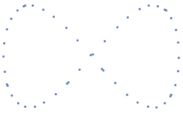
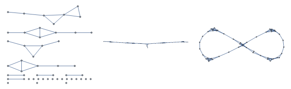
There are many ways to build a simplicial complex on top of a dataset, but one of the most common and computationally efficient method is the Vietoris-Rips complex

, which is defined as follows:

, where

is some fixed parameter--here we take

as the Euclidean distance, assuming that the dataset is embedded in some finite dimensional vector space. Essentially, we are drawing balls of radius

around each point in the dataset, and whenever there are k such balls that pairwise intersect, a k-simplex is created with those points as vertices. Take for instance the point cloud resembling the figure 8:

In[]:=

figure8=Table[{Sin[n],Sin[2n]},{n,50}]//N;ListPlot[figure8,Axes->False]

Out[]=

The Vietoris-Rips complex could be represented by a distance graph with parameter

, whose edges denote that two vertices in the dataset are within

distance of each other. Below are the distance graphs for the figure 8 with parameters 0.2, 0.3, and 0.4 (left to right):

In[]:=

DistanceGraph[data_List,epsilon_]:=If[Length[data]<=1,Graph[{}],((DistanceMatrix[data,PerformanceGoal->"Speed",DistanceFunction->EuclideanDistance]/.x_/;x>epsilon->0)/.x_/;x!=0->1)//SparseArray//AdjacencyGraph]GraphicsRow[{DistanceGraph[figure8,0.2],DistanceGraph[figure8,0.3],DistanceGraph[figure8,0.4]}]

Out[]=

We could then plug these graphs into GraphBettiNumber[]:

In[]:=

PointCloudBettiNumber[data_List,epsilon_,n_]:=GraphBettiNumber[DistanceGraph[data,epsilon],n]PointCloudBettiNumber[figure8,#,1]&/@{0.2,0.3,0.4}

Out[]=

{{25,0},{1,0},{1,2}}

Persistent Homology

Looking at the example above, one might say that the most faithful representation of the dataset is when we set

, so it makes the most sense to say that {1,2} are the actual 0th and 1st Betti numbers for the figure 8. However, this is only because we know a priori that the dataset was sampled from a figure 8, whereas in general settings we don’t really know. Therefore, a common practice in topological data analysis is to sample a range of parameters when constructing the simplicial structure, compute their respective topological features, and examine how the Betti numbers evolve.

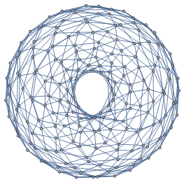
To illustrate, lets consider a set of points sampled from a donut-shaped torus:

In[]:=

donut=Join[Sequence@@Table[{(2Cos[2*π*i]+5)*Cos[2*π*j],(2Cos[2*π*i]+5)*Sin[2*π*j],2Sin[2*π*i]},{i,0,1,0.1},{j,0,1,0.05}]];ListPointPlot3D[donut]

Out[]=

We could start by playing around with different values of

to get different distance graphs, and compute their associated Betti numbers:

In[]:=

GraphicsRow[Graph[DistanceGraph[donut,#],PlotLabel->"Betti numbers:"<>ToString[PointCloudBettiNumber[donut,#,2]],LabelStyle->Directive[Bold]]&/@{1.5,2,3}]

Out[]=

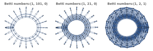
Knowing that the underlying shape is a torus, we might again say that the Vietoris-Rips complex with parameter

is the better interpolation of the dataset. Indeed, the computed Betti numbers agree with the homology groups of the actual torus (

), but that is really just cherry picking. What if our sampling of the torus was too sparse, that the dataset actually no longer represents a torus but something else? Lets try 100 evenly spaced values of

in a reasonable interval just to be sure:

In[]:=

K=ParallelMap[PointCloudBettiNumber[donut,#,2]&,Array[#&,100,{0.5,3.5}]];

In[]:=

Print["Epsilon="<>ToString[Array[#&,100,{0.5,3.5}][[#]]]<>": "<>ToString[K[[#]]]]&/@Range[1,100,10];

Epsilon=0.5: {200, 0, 0}

Epsilon=0.80303: {200, 0, 0}

Epsilon=1.10606: {143, 3, 0}

Epsilon=1.40909: {1, 101, 0}

Epsilon=1.71212: {1, 61, 0}

Epsilon=2.01515: {1, 21, 0}

Epsilon=2.31818: {1, 41, 0}

Epsilon=2.62121: {1, 2, 1}

Epsilon=2.92424: {1, 2, 1}

Epsilon=3.22727: {1, 2, 1}

The general trend is that as

gets sufficiently large, the homology of the Vietoris-Rips complex stabilizes. We could say that the topological features represented by

persists, and therefore likely encodes some intrinsic properties of the point cloud-- whereas the other features that disappeared as

gets larger do not. This is an elementary instance of persistent homology. A nice way to visualize this progression of Betti numbers is with persistence diagrams, where for each k-dimensional homological feature in the progression we record its birth and death times as an ordered pair

and plot these points on the plane:

In[]:=

birthDeathPairs[l_List,range_List]:={range[[Min[#]]],range[[Max[#]]]}&@Flatten[Position[#,1]]&/@With[{P=l/.x_Integer->Array[1&,x],m=Max[l]},(PadRight[#,m]&/@P)//Transpose]K0=birthDeathPairs[Transpose[K][[1]],Array[#&,100,{0.5,3.5}]];K1=birthDeathPairs[Transpose[K][[2]],Array[#&,100,{0.5,3.5}]];K2=birthDeathPairs[Transpose[K][[3]],Array[#&,100,{0.5,3.5}]];ListPlot[{Array[{#,#}&,10,{0.5,2.5}],K0,K1,K2},Joined->{True,False,False,False},PlotRange->Full,PlotMarkers->{False,Automatic,Automatic,Automatic},PlotLegends->{"y=x","Dimension 0","Dimension 1","Dimension 2"},AxesLabel->{"Birth","Death"},PlotStyle->{{Dashed,Black}}]

Out[]=

	y=x
	Dimension 0
	Dimension 1
	Dimension 2

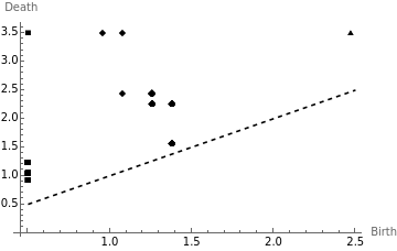
The way to read a persistence diagram is to note that the further away a point is from the diagonal line

, the longer it has persisted. In the above diagram we see that the four top most points corresponds to the actual Betti numbers of the torus.

Discrete Morse theory

When conducting topological data analysis, one issue that we quickly come up against is the sheer amount of computational demand associated with computing Betti numbers of large simplicial complexes, as we’d be required to perform row reduction on extremely large matrices. One thing one might notice is that the Vietoris-Rips complex generated from a dataset often contains many ‘redundant simplices, in that removing them would not affect the topology of the complex. Luckily, Discrete Morse theory offers us a way to ‘ignore’ the vast majority of simplices in a simplicial complex when computing their homology.

Discrete Morse functions and critical simplices

The central idea of Morse theory is to study the topological properties of smooth manifolds by looking at the critical points of a particular type of smooth function defined on the manifold. In the same spirit, the discrete analogue of Morse theory, pioneered by Robin Forman [1], seeks to study the combinatorial properties of simplicial complexes through a class of functions defined on the simplices, known as discrete Morse functions.

GraphicsRow[{Graph[CycleGraph[3],VertexLabels->{1->0,2->2,3->4},EdgeLabels->{(12)->Framed[Style["1",14,Black],Background->White,FrameStyle->White],(23)->Framed[Style["5",14,Black],Background->White,FrameStyle->White],(13)->Framed[Style["3",14,Black],Background->White,FrameStyle->White]},PlotLabel->"Valid Morse function"],Graph[CycleGraph[3],VertexLabels->{1->1,2->5,3->3},EdgeLabels->{(12)->Framed[Style["2",14,Black],Background->White,FrameStyle->White],(23)->Framed[Style["4",14,Black],Background->White,FrameStyle->White],(13)->Framed[Style["0",14,Black],Background->White,FrameStyle->White]},PlotLabel->"Invalid Morse function"]}]

Out[]=

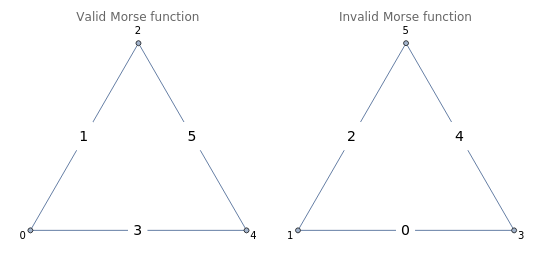
Discrete Morse functions

are maps defined on a simplicial complex

that satisfies #

and #

for all

. That is to say,

takes on strictly lower values on subsimplicies, with at most one exception per simplex. Looking at the example above (right), we see that edge and vertex labels represents an invalid Morse function, because the two endpoints of the edge labeled 0 are both assigned greater values

. We call

a critical simplex if #

and #

. For instance, the edge labeled 5 in the above example (left) represents a critical simplex, since it was assigned a higher value than all of its vertices {2,4}.

The main reason why we care about Morse functions, and in particular critical simplices, is the following: if we imagine adding-in the simplices of a simplicial complex in ascending order according to the values of a Morse function ( the sublevel sets

as we increase

), then whenever we add a non-critical simplex, it will always have a free face that is not shared by any other simplices. As such, its addition would not generate any new holes in the structure. So in a sense that will be made precise in the following sections, we only need to look at the critical simplices to determine the homology of a simplicial complex.

Gradient vector fields and acyclic matchings

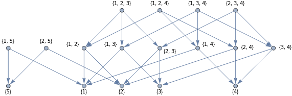
Recall that in calculus, the critical points of a differentiable real-valued function are the points where

. Given a discrete Morse function

, we associate to it a collection of arrows

indicating that

where

, which we could interpret as a gradient-like vector field. Analogous to the usual definition, the critical simplices are precisely those where this vector field vanishes. If we consider the Hasse diagram of a simplicial complex, where the simplices are partially ordered by set-inclusion, then the gradient vector field of a Morse function is represented by a modified diagram where the orientation of directed edges

are reversed whenever

. If all simplices are critical for a given Morse function, then the corresponding diagram will just be the unmodified Hasse diagram.

In[]:=

HasseDiagram[s_List]:=RelationGraph[SubsetQ[#1,#2]&&Length[Complement[#1,#2]]==1&,s,GraphLayout->"LayeredDigraphEmbedding"]S={{1},{2},{3},{4},{5},{1,5},{2,5},{1,3},{1,2},{2,3},{1,4},{2,4},{3,4},{1,2,3},{1,3,4},{1,2,4},{2,3,4}};G=Graph[HasseDiagram[S],VertexLabels->"Name"]

Out[]=

Reminiscent of the identity curl

=0 , we also have that a discrete vector field

is the gradient of a Morse function if and only if the corresponding modified Hasse diagram does not contain any non-trivial closed paths. This is seen from the fact that for a given Morse function, each simplex could at most be incident to one gradient vector (regardless of orientation), thus the gradient vector field corresponds to a partial matching of the Hasse diagram. Suppose for some n-simplex

there exists a nontrivial directed cycle

of length

, and let

be a partial matching corresponding to a gradient vector field. Since each edge

ascends to a simplex of dimension +1, and each edge

descends to a simplex of dimension -1, we must have that #

for the

edges in the path. Since it is impossible for two consecutive edges to appear in a matching, this implies that the cycle alternates between edges in

and edges not in

. This directly gives us the chain

, where the inequalities are strict in an alternating fashion--a contradiction. Conversely, since a digraph has a topological ordering (an indexing of the vertex set satisfying

is an edge only if

) if it is acyclic, given an acyclic partial matching

we know that the corresponding modified Hasse diagram will induce such an ordering on the set of simplices. Then

(or any monotonically decreasing function in k) is a discrete Morse function whose gradient is

. Conveniently, Mathematica has a built-in function for finding topological orderings, which will come in handy later on:

TopologicalSort[HasseDiagram[S]]

Out[]=

{{2,3,4},{1,2,4},{2,4},{1,3,4},{3,4},{1,4},{4},{1,2,3},{2,3},{1,2},{1,3},{3},{2,5},{2},{1,5},{5},{1}}

In practice, what this means is that we don’t have to explicitly work with Morse functions--all we need is an acyclic partial matching of the Hasse diagram to identify the critical simplices of a Morse function.

Morse Homology

As hinted at in previous sections, critical simplices in some sense determine the homology of the simplicial complex. More precisely, if we define

to be the linear span (with integer coefficients) of dimension-k critical simplices , then we have boundary operators

inducing homology groups

that are isomorphic to the usual ones. We define the boundary maps on the basis elements as follows, and extend linearly:

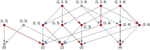
Where

are direct paths in the modified Hasse diagram from a face of

to a k-1 critical simplex

, and

encodes the orientation that

induces on

. For our purposes, we consider homology groups with coefficients in

, which won’t really cause problems barring certain technicalities (see Universal Coefficient Theorem). Then the sum

is simply zero if there are an even number of gradient paths from

, and 1 otherwise. As a sanity check of why the Morse boundary operators

on the Morse complex would actually gives rise to the same homology groups as induced by the classical ones, notice that if we have an empty Morse matching, then every simplex is critical. Moreover, the only element of

will be the trivial path from a face to itself, in which case

clearly degenerates to

. The next best thing to a proof is a concrete example. We start by finding a valid Morse matching for the following Hasse diagram:

In[]:=

M={{1,5}{1},{1,2}{2},{1,3}{3},{2,4}{4},{1,2,3}{2,3},{1,3,4}{1,4},{2,3,4}{3,4}};HighlightGraph[G,Graph[M]]

Out[]=

In[]:=

EdgeReverse[G_Graph,M_List]:=EdgeAdd[EdgeDelete[G,M],Reverse[#]&/@M]modifiedDiagram=EdgeReverse[G,M];modifiedDiagram//AcyclicGraphQ

Out[]=

False

The critical simplices are then the unmatched vertices (in this case there is precisely one in each dimension):

In[]:=

CriticalSimplicies=Complement[VertexList[G],VertexList[Graph[M]]]

Out[]=

{{5},{2,5},{1,2,4}}

We could then simply count the number of paths going from one critical simplex to another, and determine their parity:

In[]:=

DegreeSum[s1_,s2_,G_]:=With[{P=FindPath[G,s1,s2,Infinity,All]},If[EvenQ[P//Length],0,1]]//N

In this case, no paths going from

exist, and there are two such paths going from

HighlightGraph[modifiedDiagram,Subgraph[G,Union[FindPath[modifiedDiagram,{2,5},{5},Infinity,All]]]]

Out[]=

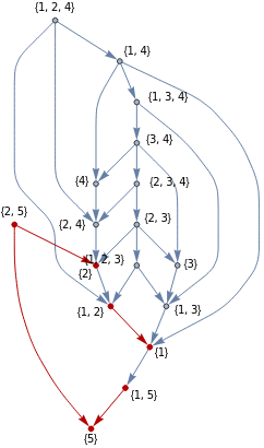
DegreeSum[{2,5},{5},modifiedDiagram]

Out[]=

This tells us that the Morse boundary operators are all trivial, meaning that

for all

, thus the homology groups of this simplicial complex is simply

for all other

. This agrees with what we have originally found at the very beginning of the article, i.e.

Generating Morse matchings

As seen from the above example, having a Morse matching that minimizes the number of critical simplices will make calculating Betti numbers significantly more straightforward. Ideally, we’d want to have a computationally efficient algorithm of searching for such matchings. We start by finding a topological ordering of the initial Hasse diagram, and proceed with a greedy algorithm starting at the lowest dimensional simplex in the ordering that iteratively checks if each simplex could be matched with another without creating cycles:

In[]:=

EdgeToList[E_]:=Union[Sequence@@(E/.DirectedEdge[v_,w_]->{v,w})]validMatching[g_,m_,M_]:=AcyclicGraphQ[EdgeReverse[g,{m}]]&&Intersection[EdgeToList[{m}],EdgeToList[M]]=={}InitialMatching[G_Graph]:=Module[{g=G,ordering=TopologicalSort[G]//Reverse,M={}},i=1;While[i<=Length[ordering],With[{match=FirstCase[IncidenceList[g,ordering[[i]]],x_/;validMatching[g,x,M],Nothing]},M=Append[M,match];g=EdgeReverse[g,{match}]];i++];M]

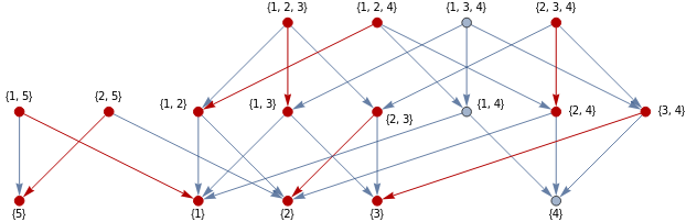
In simple cases, this algorithm is already sufficient for finding the optimal matching. For instance, with the same example as previously, it produced a matching that again leaves one critical simplex per dimension:

HighlightGraph[G,Graph[InitialMatching[G]]]H=EdgeReverse[G,InitialMatching[G]];H//AcyclicGraphQ

Out[]=

True

And as expected, the Morse boundary operators are also trivial in this new matching:

Print[DegreeSum[{1,4},{4},H]]Print[DegreeSum[{1,3,4},{1,4},H]]

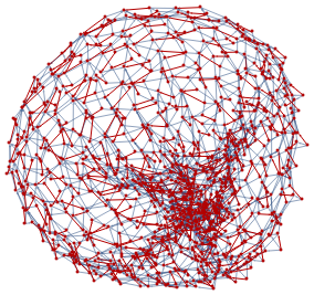
We turn our attention to a slightly more complicated example-a triangulation of the torus:

In[]:=

torusIdentifications[n_,m_]:=Join[N[{{1,#},{m,#}}&/@Range[1,n]],N[{{#,1},{#,n}}&/@Range[1,m]]]torusGrid[n_,m_]:=Graph[VertexContract[diagonalGridGraph[n,m],torusIdentifications[n,m]],VertexCoordinates->Automatic]torusGrid[15,15]T=Sort[#]&/@GraphComplex[torusGrid[15,15],2];diagram=HasseDiagram[T];GraphBettiNumber[torusGrid[15,15],2]

Out[]=

{1,2,1}

Our greedy algorithm indeed produced a valid Morse matching:

In[]:=

matching=InitialMatching[diagram];HighlightGraph[Graph[diagram],Graph[matching],GraphLayout->"HighDimensionalEmbedding"]H=EdgeReverse[diagram,matching];H//AcyclicGraphQ

Out[]=

True

We then find that the Morse boundary operators all vanish:

In[]:=

criticalSimplices=Sort[Complement[VertexList[diagram],EdgeToList[matching]]]

Out[]=

{{{14.,14.}},{{1.,14.},{14.,14.}},{{14.,1.},{14.,14.}},{{1.,1.},{1.,14.},{2.,14.}}}

DegreeSum[{{1.`,1.`},{1.`,14`},{2.`,14.`}},{{14.`,1.`},{14.`,14.`}},H]//PrintDegreeSum[{{1.`,1.`},{1.`,14`},{2.`,14.`}},{{1.`,14.`},{14.`,14.`}},H]//PrintDegreeSum[{{14.`,1.`},{14.`,14.`}},{{14.`,14.`}},H]//PrintDegreeSum[{{1.`,14.`},{14.`,14.`}},{{14.`,14.`}},H]//Print

Thus agreeing with the Betti numbers of the torus.

Of course, the greedy algorithm likely won’t be very effective when dealing with more complicated simplicial complexes, such as those arising from large datasets. One result that might be useful is the following [1]--given an acyclic directed graph, if there exists a unique path from

, then reversing the orientation of all edges in the path will not create any directed cycles. This in particular implies that given a Morse matching, if we can find a unique gradient path from an

-critical simplex

to an

-critical simplex

, then we can obtain a modified Morse matching with the same critical simplices by reversing the orientation of all edges in the path, except now

are no longer critical:

g=Graph[{1->2,2->3,3->4,4->5,5->6},VertexCoordinates->{{0,0.5},{1,0},{2,0.5},{3,0},{4,0.5},{5,0}},VertexLabels->{1->v,6->w}];h=Graph[{6->5,5->4,4->3,3->2,2->1},VertexCoordinates->{{5,0},{4,0.5},{3,0},{2,0.5},{1,0},{0,0.5}},VertexLabels->{1->v,6->w}];GraphicsRow[{HighlightGraph[g,Graph[{2->3,4->5}]],Graphics[{Thick,{Arrowheads[Medium],Arrow[{{0,0},{0.5,0}}]}}],HighlightGraph[h,Graph[{2->1,4->3,6->5}]]},ImageSize->Medium]

Out[]=

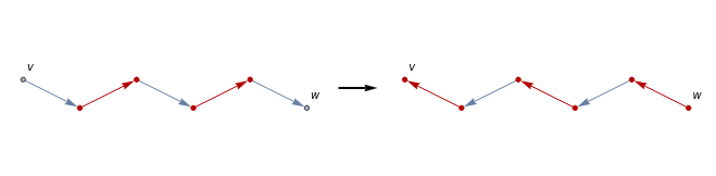
Using this idea of cancelling critical simplices, one could generate an initial matching on a given Hasse diagram using something like the greedy algorithm as demonstrated above, then proceed to iteratively check for the existence of such paths to further augment the matching if the initial matching wasn’t maximal.

Concluding remarks

This computational essay was in many ways a continuation to the project I did for WS22, where I explored the behavior of cellular automaton on various topological surfaces, as it sparked my interest in exploring the computable aspects of topology.

Needless to say, I’ve barely scratched the surface of computational topology and discrete Morse theory--there’s just so much more to be explored, such as finding a fast algorithm for generating Vietoris-Rips complexes on datasets and optimal Morse matchings, or using TDA to feature engineer data in a machine learning pipeline, or simulating dynamical systems on simplicial complexes, etc. What fascinates me about these topics is that they turn esoteric mathematics into a common playground, where people who are interested in different things could find their own way of playing around with ideas in these rich theories that would otherwise only have been known to and appreciated by a very small minority of people.

Please feel free to point out any mistakes that you spot. I’d also like to thank Rory and my advisor Isabel for all the help they’ve given me, as well the people who’ve made the WELP program possible.

References

Robin Forman, A user’s guide to Discrete Morse Theory

Frederic Chazal et al. , An Introduction to Topological Data Analysis: Fundamental and Practical Aspects for Data Scientists

CITE THIS NOTEBOOK

Introduction to Persistent Homology and Discrete Morse Theory
by Shuheng Li
Wolfram Community, STAFF PICKS, August 30, 2023
https://community.wolfram.com/groups/-/m/t/3001504