Rational polarization and ambiguous evidence: models and simulations
by Kevin Dorst
kevindorst@pitt.edu
October 2021
by Kevin Dorst
kevindorst@pitt.edu
October 2021
General frame functions (run this first):
General frame functions (run this first):
Overview:
Overview:
This notebook contains the code needed to run all simulations presented in the manuscript "Rational Polarization". It is meant to be read in tandem with Appendix C of that paper.
As explained in the paper, the goal is to show how ambiguous-evidence models that satisfy the value of evidence can nevertheless lead to predictable polarization.
It is divided into three sections.
0) General introduction
1) Cognitive Search models — Provides the models used in §6 of the paper on confirmation bias, along with robustness checks.
2) Argument models — Provides the simple model used in §7 of the paper on the group polarization effect, along with robustness checks.
3) Combined models — Provides the combined model of arguments and scrutiny used in §7, along with robustness checks.
NOTE: sections (1) and (2) are independent, but (3) requires that the functions from (1) and (2) already be loaded (you do not need to run the simulations from (1) and (2) to run section (3); just initialize the functions csQModel, getArgModel, etc.).
Any questions about or problems with the code, please let me know! Email me at kevindorst@pitt.edu
0) General Introduction
0) General Introduction
The models used in this notebook (and in the paper) are known as probability frames, and are modeled with (row-)stochastic matrices. (See e.g. here for a summary.) An NxN matrix M represents a model with n worlds, and M(i,j) represents the probability that world i assigns to world j. (Note: the interpretation is different than standard Markov chains; we are not modeling the probability of transitioning to another state; we are modeling the probability of currently being in another state.)
The N worlds, W={1,2,...,N} are thought of as a partition of logical space, so subsets of {1,2...N} are events or propositions. Even E ⊆ W is true at world i iff i ∈ E. The probability function P_i associated with world i (and encoded in row i) captures the rational opinions to adopt if you are in fact in world i. Notice, following standard epistemic logic, that this allows us to define events about rational probabilities as events in the frame: given an eventE, the event [P(E) = 1/2] is simply the set of worlds i at which P_i(E) = 1/2. So for any E ⊆ W and t between 0 and 1: [P(E) = t] := {i ∈W: P_i(E) = t}. This allows us to “unravel” higher-order probability claims of any order as simply claims about probabilities of events.
In standard Bayesian models, probabilities are introspective meaning that if P_i is the rational credence to adopt at a given world i, then P_i is certain that it’s at a world where P_i is the rational credence function. Thus the validate the axiom [P(E) =t] –> [P(P(E)=t)=1]. Such models are equivalent to block-diagonal matrices in which block has the same probabilities.
For example, suppose we start with a given prior over 6 worlds:
In[]:=
prior=getRandProbVec[4]//N
Out[]=
{0.1,0.4,0.4,0.1}
Then suppose the posterior probabilities are obtained by conditioning this prior on the true member of the partition {{1,2},{3,4}}. This yields the resulting model:
In[]:=
MatrixForm[frame=Join[Table[condition[prior,{1,2}],2],Table[condition[prior,{3,4}],2]]]
Out[]//MatrixForm=
0.2 | 0.8 | 0. | 0. |
0.2 | 0.8 | 0. | 0. |
0. | 0. | 0.8 | 0.2 |
0. | 0. | 0.8 | 0.2 |
If we wanted to represent this entire update in single object, we can treat the prior as the first row of the matrix, assigned probability 0 by all worlds, like so:
In[]:=
MatrixForm[updateFrame=Prepend[#,0]&/@Join[{prior},frame]]
Out[]//MatrixForm=
0 | 0.1 | 0.4 | 0.4 | 0.1 |
0 | 0.2 | 0.8 | 0. | 0. |
0 | 0.2 | 0.8 | 0. | 0. |
0 | 0. | 0. | 0.8 | 0.2 |
0 | 0. | 0. | 0.8 | 0.2 |
So the worlds of our model are now {2,3,...,N+1}. I’ll write update in this way in all the models that follow.
Notice that in the above model, the posterior probabilities (rows 2–4) are introspective in the sense that if P_i(j)>0, then P_j = P_i: if the rational posterior probabilities at world i leave open world j, then the rational posterior probabilities at world j are the same as those at world i.
When that condition fails, evidence is ambiguous in the sense used in the paper. For example, here’s a matrix that represents an update from a prior to one of two rational posteriors, but in which those rational posteriors are unsure what the rational posteriors are. In particular, they are gotten by “Jeffrey-shifting” the prior in two different ways at the different worlds:
When that condition fails, evidence is ambiguous in the sense used in the paper. For example, here’s a matrix that represents an update from a prior to one of two rational posteriors, but in which those rational posteriors are unsure what the rational posteriors are. In particular, they are gotten by “Jeffrey-shifting” the prior in two different ways at the different worlds:
post1=condition[prior,{1,2}];post2=condition[prior,{3,4}];MatrixForm[ambFrame=Join[Table[jShift1=0.75post1+0.25post2,2],Table[jShift2=0.25post1+0.75post2,2]]]
Out[]//MatrixForm=
0.15 | 0.6 | 0.2 | 0.05 |
0.15 | 0.6 | 0.2 | 0.05 |
0.05 | 0.2 | 0.6 | 0.15 |
0.05 | 0.2 | 0.6 | 0.15 |
We can again put this entire update in a single matrix:
In[]:=
MatrixForm[ambUpdate=Prepend[#,0]&/@Join[{prior},ambFrame]]
Out[]//MatrixForm=
0 | 0.1 | 0.4 | 0.4 | 0.1 |
0 | 0.15 | 0.6 | 0.2 | 0.05 |
0 | 0.15 | 0.6 | 0.2 | 0.05 |
0 | 0.05 | 0.2 | 0.6 | 0.15 |
0 | 0.05 | 0.2 | 0.6 | 0.15 |
Notice two things.
1) First, in this frame the posterior probabilities are not introspective. The probability function associated world 2, P_2, assigns positive probability to world 4, yet P_2 ≠ P_4. Thus, if world 2 is actual, then the probabilities that are in fact rational (P_2) do not know that they are in fact rational—they leave open that some different probabilities (P_4) are rational.
2) Second, even though this frame is not introspective, the update is still valuable in the sense defined in (§2 of) the “Rational Polarization” paper: there is no Dutch book against transitioning from the prior to the posterior, i.e. the prior expects the posterior to be more accurate on every strictly proper scoring rule, i.e. the prior expects the posterior to make a better choice for any decision problem. See this paper for further discussion. We can use one of the functions from that paper’s notebook to verify that the above frame is in fact “valuable” in this sense:
In[]:=
checkTotalTrust[ambUpdate]
Out[]=
{True}
With that preamble, I’ll move on to explaining how such valuable, ambiguous-evidence updates can nevertheless lead to predictable polarization.
1) Cognitive Search Models
1) Cognitive Search Models
The csQModel function generates a cognitive search model with a given set of parameters. There are a variety of ways to parameterize such models, but this function so by taking the prior probability of q (priorQ) the extent to which this goes up conditional on there being a flaw (gBump π(q|F) - π(q)), the prior probability of finding a flaw (priorGG = π(F)), the prior probability of there being a flaw that you don’t find (priorGB = π(C)), the prior probability of there being no flaw (priorBB = π(N)), the posterior probability that P assigns to N, if N obtains (postBB = P_x(N), for x in N), and the posterior probability that P assigns to C, if C obtains (postGB = P_y(C), for y\in C).
NOTES:
– the set of worlds {2,4,6} represents the proposition q; {2,3} are N, {4,5} are C, and {6,7} are F. 1 is an invisible world that encode the prior.
– The function csQModel can take any (probabilistic) parameters and will output a corresponding model; it’ll output Error if the parameters force the certain parts of the model to be non-probabilistic.
In[]:=
(*note:q={2,4,6}*)csQModel[priorQ_,gBump_,priorGG_,priorGB_,priorBB_,postGB_,postBB_]:=(qGivenG=priorQ+gBump;(*SeewhatprobofqgivenBBmustbe*)qGivenB=var78/.Flatten[Solve[priorQpriorBB*var78+(priorGG+priorGB)(priorQ+gBump),var78]];If[qGivenB<0||qGivenB>1,Return["Error"]];Return[{(*prior:*){0,priorBB*qGivenB,priorBB(1-qGivenB),priorGB*qGivenG,priorGB(1-qGivenG),priorGG*qGivenG,priorGG*(1-qGivenG)},(*BBprobs:*){0,postBB*qGivenB,postBB*(1-qGivenB),(1-postBB)qGivenG,(1-postBB)(1-qGivenG),0,0},{0,postBB*qGivenB,postBB*(1-qGivenB),(1-postBB)qGivenG,(1-postBB)(1-qGivenG),0,0},(*GBprobs:*){0,(1-postGB)*qGivenB,(1-postGB)*(1-qGivenB),(postGB)qGivenG,(postGB)(1-qGivenG),0,0},{0,(1-postGB)*qGivenB,(1-postGB)*(1-qGivenB),(postGB)qGivenG,(postGB)(1-qGivenG),0,0},(*GGprobs:*){0,0,0,0,0,qGivenG,1-qGivenG},{0,0,0,0,0,qGivenG,1-qGivenG}}])
This outputs a frame in stochastic-matrix notation, where row i column j equals P_i(j). We treat world 1 as a “dummy” world that no world assigns positive probability to, and its probability function encodes the prior over the rest of the frame.
For example, here is what we get if the prior in q is 0.5, the bump if you find a flaw is 0.5, the prior probability of doing so is 0.25, the prior probability of there being a flaw you fail to find is 0.25, the prior probability of there not being a flaw is 0.5, the posterior rational confidence there’s no flaw, if there is no flaw is 2/3, and the posterior rational confidence there is a flaw, if there is a flaw that you don’t find is also 2/3:
For example, here is what we get if the prior in q is 0.5, the bump if you find a flaw is 0.5, the prior probability of doing so is 0.25, the prior probability of there being a flaw you fail to find is 0.25, the prior probability of there not being a flaw is 0.5, the posterior rational confidence there’s no flaw, if there is no flaw is 2/3, and the posterior rational confidence there is a flaw, if there is a flaw that you don’t find is also 2/3:
In[]:=
frame=csQModel[0.5,0.5,0.25,0.25,0.5,2/3,2/3]
Out[]=
{{0,0.,0.5,0.25,0.,0.25,0.},{0,0.,0.666667,0.333333,0.,0,0},{0,0.,0.666667,0.333333,0.,0,0},{0,0.,0.333333,0.666667,0.,0,0},{0,0.,0.333333,0.666667,0.,0,0},{0,0,0,0,0,1.,0.},{0,0,0,0,0,1.,0.}}
In[]:=
MatrixForm[frame]
Out[]//MatrixForm=
0 | 0. | 0.5 | 0.25 | 0. | 0.25 | 0. |
0 | 0. | 0.666667 | 0.333333 | 0. | 0 | 0 |
0 | 0. | 0.666667 | 0.333333 | 0. | 0 | 0 |
0 | 0. | 0.333333 | 0.666667 | 0. | 0 | 0 |
0 | 0. | 0.333333 | 0.666667 | 0. | 0 | 0 |
0 | 0 | 0 | 0 | 0 | 1. | 0. |
0 | 0 | 0 | 0 | 0 | 1. | 0. |
Notice that this is just the coarse-grained word-completion model specified in Figure 2 in the paper.
If we change the gBump to be less than 0.5, we get a less extreme example:
If we change the gBump to be less than 0.5, we get a less extreme example:
In[]:=
frame=csQModel[0.5,0.2,0.25,0.25,0.5,2/3,2/3]
Out[]=
{{0,0.15,0.35,0.175,0.075,0.175,0.075},{0,0.2,0.466667,0.233333,0.1,0,0},{0,0.2,0.466667,0.233333,0.1,0,0},{0,0.1,0.233333,0.466667,0.2,0,0},{0,0.1,0.233333,0.466667,0.2,0,0},{0,0,0,0,0,0.7,0.3},{0,0,0,0,0,0.7,0.3}}
In[]:=
MatrixForm[frame]
Out[]//MatrixForm=
0 | 0.15 | 0.35 | 0.175 | 0.075 | 0.175 | 0.075 |
0 | 0.2 | 0.466667 | 0.233333 | 0.1 | 0 | 0 |
0 | 0.2 | 0.466667 | 0.233333 | 0.1 | 0 | 0 |
0 | 0.1 | 0.233333 | 0.466667 | 0.2 | 0 | 0 |
0 | 0.1 | 0.233333 | 0.466667 | 0.2 | 0 | 0 |
0 | 0 | 0 | 0 | 0 | 0.7 | 0.3 |
0 | 0 | 0 | 0 | 0 | 0.7 | 0.3 |
The getBBCondQCSModel generates a random cognitive-search model by taking in a prior probability for q, qPrior, the change in probability for q that would result from finding a flaw, gBump, and the probability of finding a word, fprob, and generating a random cognitive search model by (1) pulling a probability of there being a flaw (priorW) randomly from [0,1], and then (2) using these parameters to generate a cognitive search model by setting the posterior probability if there’s no word to be the result of conditioning on not finding one, and setting the posterior probability if there is a word you don’t find to assign at least as high probability to there being a flaw as that---as required by Value.
In[]:=
getBBCondQCSModel[qPrior_,gBump_,fprob_]:=halt=False;(*num=0;*)WhilehaltFalse,priorW=RandomReal[{0,1}];condBBconf=;postBBconf=condBBconf;postGBconf=RandomReal[{1-condBBconf,1}];priorGG=priorW*fprob;priorGB=priorW*(1-fprob);priorBB=1-priorW;(*num+=1;*)(*Keeprepeatingtillgetparametersthatyieldalegitframe:*)If[StringQ[csQModel[qPrior,gBump,priorGG,priorGB,priorBB,postGBconf,postBBconf]]False,halt=True];;Return[csQModel[qPrior,gBump,priorGG,priorGB,priorBB,postGBconf,postBBconf]];
1-priorW
1-priorW+priorW(1-fprob)
This outputs a frame in stochastic-matrix notation, where row i column j equals P_i(j). For example:
In[]:=
getBBCondQCSModel[0.5,0.2,0.5]
Out[]=
{{0,0.165681,0.35672,0.167159,0.0716398,0.167159,0.0716398},{0,0.217658,0.468629,0.2196,0.0941141,0,0},{0,0.217658,0.468629,0.2196,0.0941141,0,0},{0,0.0374131,0.0805525,0.617424,0.26461,0,0},{0,0.0374131,0.0805525,0.617424,0.26461,0,0},{0,0,0,0,0,0.7,0.3},{0,0,0,0,0,0.7,0.3}}
In[]:=
MatrixForm[%]
Out[]//MatrixForm=
0 | 0.165681 | 0.35672 | 0.167159 | 0.0716398 | 0.167159 | 0.0716398 |
0 | 0.217658 | 0.468629 | 0.2196 | 0.0941141 | 0 | 0 |
0 | 0.217658 | 0.468629 | 0.2196 | 0.0941141 | 0 | 0 |
0 | 0.0374131 | 0.0805525 | 0.617424 | 0.26461 | 0 | 0 |
0 | 0.0374131 | 0.0805525 | 0.617424 | 0.26461 | 0 | 0 |
0 | 0 | 0 | 0 | 0 | 0.7 | 0.3 |
0 | 0 | 0 | 0 | 0 | 0.7 | 0.3 |
The function getGlobPartitionInAcc gets the Brier inaccuracy of P_w at a given world w in a frame as described Appendix C:
getGlobPartitionInAcc[frame_,world_]:=size=Length[frame];singletons=({#1}&)/@Range[size];ReturnTotal&/@singletons
2
(probability[frame〚world〛,#1]-truth[world,#1])
size
We can use this to test the correlation between π(Find | Flaw) and the expected accuracy of the update, as described in §6 and Appendix C of the paper. To minimize unnecessary variance, we fix a
In[]:=
numTrials=10000;qPrior=0.5;results=Reap[Do[gBump=RandomReal[{0,Min[{0.2,1-qPrior}]}];pFind=RandomReal[{0,1}];frame=getBBCondQCSModel[qPrior,gBump,pFind];size=Length[frame];prior=frame[[1]];expPrior=MatrixPower[frame,2][[1]];inAccVec=getGlobPartitionInAcc[frame,#]&/@Range[size];accVec=1-inAccVec;(*ambVec=getGlobPartitionSdAmb[frame,#]&/@Range[size];*)Sow[{pFind,prior.accVec}],numTrials]][[2,1]];
We can fit a linear model to the result to see how well changes in π(Find|Flaw) explain the variance in expected accuracy, and plot the results:
In[]:=
lm=LinearModelFit[results,x,x];lm["RSquared"]Show[ListPlot[results,PlotStyleOpacity[0.5],Frame{{True,False},{True,False}},ImageSizeLarge,FrameLabel{{Style["Expected Accuracy",FontSize14],None},{Style["Chance of finding if there is a flaw; π(Find|Flaw)",FontSize14],None}},FrameTicksAll,FrameTicksStyleDirective[FontSize14]],Plot[Normal[lm],{x,0,1},PlotStyleThick]]
Out[]=
0.422777
Out[]=
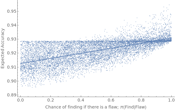
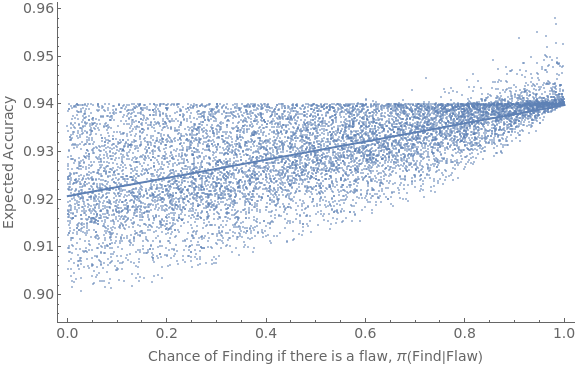
Similar results happen if we use different priors in q and/or different range in the size of gBumps:
In[]:=
numTrials=10000;qPrior=0.7;results=Reap[Do[gBump=RandomReal[{0,Min[{0.1,1-qPrior}]}];pFind=RandomReal[{0,1}];frame=getBBCondQCSModel[qPrior,gBump,pFind];size=Length[frame];prior=frame[[1]];expPrior=MatrixPower[frame,2][[1]];inAccVec=getGlobPartitionInAcc[frame,#]&/@Range[size];accVec=1-inAccVec;(*ambVec=getGlobPartitionSdAmb[frame,#]&/@Range[size];*)Sow[{pFind,prior.accVec}],numTrials]][[2,1]];
In[]:=
lm=LinearModelFit[results,x,x];lm["RSquared"]Show[ListPlot[results,PlotStyleOpacity[0.5],Frame{{True,False},{True,False}},ImageSizeLarge,FrameLabel{{Style["Expected Accuracy",FontSize14],None},{Style["Chance of Finding if there is a flaw, π(Find|Flaw)",FontSize14],None}},FrameTicksAll,FrameTicksStyleDirective[FontSize14]],Plot[Normal[lm],{x,0,1},PlotStyleThick]]
Out[]=
0.393123
Out[]=
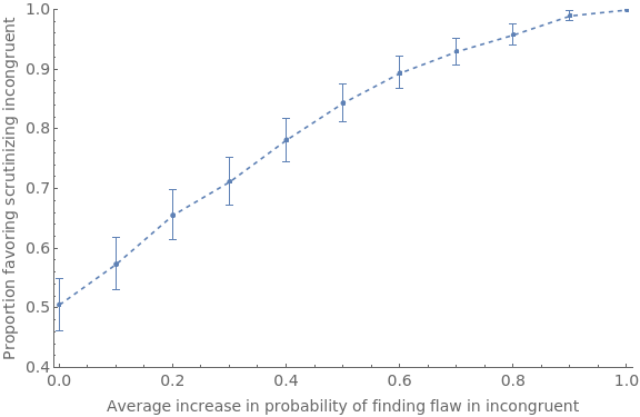
Given this, we want to simulate how often expected accuracy will lead you to prefer to scrutinize incongruent studies over congruent ones, as a function of how much more likely (on average) you are to find flaws in the former. We fix a given prior, and then let pBump be a parameter that puts a minimum on how likely you are to find a flaw in the incongruent study, and 1–pBump gives the maximum of how likely you are to find a flaw in the congruent study. By letting pBump vary from 0, to 0.1, ... to 1, and within each generating 500 pairs and recording the proportion which have higher expected accuracy for scrutinizing the incongruent study, we see that the degree of selective scrutiny increases with this rate:
In[]:=
Needs["HypothesisTesting`"]
In[]:=
Clear[rate];Clear[results];qPrior=0.5;Do[pBump=iter;results[iter]=Reap[Do[(*pFind2isaboveonaverage*)pFind1=RandomReal[{0,1-pBump}];pFind2=RandomReal[{0+pBump,1}];gBump1=RandomReal[{0,Max[{-0.2,-qPrior}]}];gBump2=RandomReal[{0,Min[{0.2,1-qPrior}]}];frame1=getBBCondQCSModel[qPrior,gBump1,pFind1];frame2=getBBCondQCSModel[qPrior,gBump2,pFind2];size=Length[frame1];prior1=frame1[[1]];inAccVec1=getGlobPartitionInAcc[frame1,#]&/@Range[size];accVec1=1-inAccVec1;expAcc1=prior1.accVec1;size=Length[frame2];prior2=frame2[[1]];inAccVec2=getGlobPartitionInAcc[frame2,#]&/@Range[size];accVec2=1-inAccVec2;expAcc2=prior2.accVec2;Sow[expAcc2>expAcc1];,500]][[2,1]];results[iter]=results[iter]/.{True1,False0};rate[iter]=Total[results[iter]]/Length[results[iter]]//N,{iter,0,1,0.1}]rateSeq={#,Around[Interval[MeanCI[results[#]]]]}&/@Range[0,1,0.1];ListLinePlot[rateSeq,PlotStyleDashed,PlotMarkersAutomatic,PlotRange{{-0.01,1.01},{.4,1}},ImageSizeLarge,Frame{{True,False},{True,False}},FrameLabel{{Style[StringForm["Proportion favoring scrutinizing incongruent"],FontSize14],None},{Style[StringForm["Average increase in probability of finding flaw in incongruent"],FontSize14],None}},FrameTicks{{Automatic,Automatic},{Automatic,Automatic}},FrameTicksStyleDirective[FontSize14]]
Out[]=
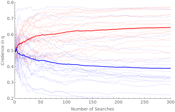
We’re now in a position to simulate what happens when two groups of agents are presented with a series of pairs of studies to scrutinize. One group (red) is on average better at finding flaws in the studies that tells against q; the other group (blue) is on average better at finding flaws in studies that tell in favor of q. There are a variety of choice-points in the simulation; see Appendix C for some discussion.
Note certain finicky things about this simulation:
– Strange things happen when the minpFind and maxpFind are allowed to go all the way to 0 and 1; this may be simply from non-linearities which lead to massive drops in credence when you fail to find a flaw, OR it may be an error in the code which I’ve been unable to locate
– Although increasing findGap generally increases the degree of polarization, it is not quite linear—and as it gets very large (0.8 or 0.9) the polarization starts to shrink a bit—perhaps due to the same issue that causes the above issue when minpFind and maxpFind are too extreme.
– Note that “confGBump”, “confpFind”, etc. refer to parameters of the study that is expectably confirmatory for q, meaning that if a flaw is found it RAISES the credence in q. Thus it does NOT refer to the study that confirms q, and in which finding a flw would lead you to lower your credence in q. Vice versa for disConfGBump, etc.
q={2,4,6};numSearches=300;numAgents=20;(*rateatwhichopinionssolidify/changelessateachupdate:*)hardenSpeed=0.5;(*differentialprobabilitiesoffindingerrors;between0–0.8:*)findGap=0.5;minpFind=0.1;maxpFind=0.9;Timing[Do[iter;Do[agIter;If[iter"pro",ag[agIter,est]=0.5];If[iter"con",ag[agIter,est]=0.5];ag[agIter,weight]=10;newTraj[agIter,iter]=Reap[Do[(*getthepFindsforstudy*)If[iter"pro",confpFind=RandomReal[{minpFind+findGap,maxpFind}];disConfpFind=RandomReal[{minpFind,maxpFind-findGap}];];If[iter"con",confpFind=RandomReal[{minpFind,maxpFind-findGap}];disConfpFind=RandomReal[{minpFind+findGap,maxpFind}];];;(*Sethowfarmightshiftopinionateachstage:*)range=Min[ag[agIter,est],1-ag[agIter,est]];confGBump=(RandomReal[{0,range}]/(hardenSpeed*ag[agIter,weight]));disConfGBump=(RandomReal[{-range,0}]/(hardenSpeed*ag[agIter,weight]));frameS1=getBBCondQCSModel[ag[agIter,est],confGBump,confpFind];frameS2=getBBCondQCSModel[ag[agIter,est],disConfGBump,disConfpFind];inAccVecS1=getGlobPartitionInAcc[frameS1,#]&/@Range[Length[frameS1]];inAccVecS2=getGlobPartitionInAcc[frameS2,#]&/@Range[Length[frameS2]];expInAccS1=frameS1[[1]].inAccVecS1;expInAccS2=frameS2[[1]].inAccVecS2;If[expInAccS1≤expInAccS2,chosenFrame=frameS1;chosenPFind=confpFind;,chosenFrame=frameS2;chosenPFind=disConfpFind;];priorG=probability[chosenFrame[[1]],{4,5,6,7}];If[RandomVariate[BernoulliDistribution[priorG]]1,(*makeposteriorGG,withchancematchingpFindS1*)If[RandomVariate[BernoulliDistribution[chosenPFind]]1,(*MakeposteriorGG*)ag[agIter,est]=probability[chosenFrame[[6]],q];ag[agIter,weight]+=1;,(*ifdon'tfind,posteriorisGB*)ag[agIter,est]=probability[chosenFrame[[4]],q];ag[agIter,weight]+=1];,(*makeposteriorBB*)ag[agIter,est]=probability[chosenFrame[[2]],q];;ag[agIter,weight]+=1];Sow[{ag[agIter,weight]-10,ag[agIter,est]}];,numSearches]][[2,1]];,{agIter,numAgents}],{iter,{"pro","con"}}]]proTrajs=newTraj[#,"pro"]&/@Range[numAgents];avgProTraj=Mean[proTrajs];conTrajs=newTraj[#,"con"]&/@Range[numAgents];avgConTraj=Mean[conTrajs];Show[ListLinePlot[proTrajs,PlotStyleDirective[Red,Opacity[0.1]],PlotRange{{0,numSearches},{0.2,0.8}},Frame{{True,False},{True,False}},ImageSizeLarge,FrameLabel{{Style["Credence in q",FontSize14],None},{Style["Number of Searches",FontSize14],None}},FrameTicksAll,FrameTicksStyleDirective[FontSize14]],ListLinePlot[avgProTraj,PlotStyleDirective[Red,Thick]],ListLinePlot[conTrajs,PlotStyleDirective[Blue,Opacity[0.1]]],ListLinePlot[avgConTraj,PlotStyleDirective[Blue,Thick]]]
Out[]=
{31.537,Null}
Out[]=
Robustness checks
Robustness checks
2) Argument models
2) Argument models
The getArgModel function generates an argument model with a given set of parameters. It takes the prior probability of q (priorQ), the probability of q if the argument is good (gInf), the confidence you should have THAT the argument is good if indeed it is (gConf), the probability of q if the argument is bad (bInf), and the confidence you should have THAT the argument is bad if indeed it is (bConf).
NOTES:
– {2,4} represents the proposition q.
– Given the constraints, the function solves for the prior probability of G, π(G). In order to satisfy the value of evidence, we must have gConf ≥ π(G) and bConf ≥ π(G) = 1 – π(G). If the parameters you input violate this constraint, the function will output an Error.
– Make sure the input parameters are all between 0 and 1
– This function WILL allow you to make the argument more ambiguous if it’s bad (B = {4,5}) than if it’s good (G = {2,3}); but that would violate its intended interpretation.
In[]:=
getArgModel[priorQ_,gInf_,gConf_,bInf_,bConf_]:=(*{2,4}istheclaimq*)((*getpriorconfidencethatingoodcase:*)priorG=x/.Solve[priorQx*(gInf)+(1-x)(bInf),x][[1]];If[priorG>gConf,Print["gConf below priorG"]];If[1-priorG>bConf,Print["bConf below 1-priorG"]];(*Generateframe:*)Return[{{0,priorG*gInf,priorG*(1-gInf),(1-priorG)(bInf),(1-priorG)(1-bInf)},{0,gConf*gInf,gConf(1-gInf),(1-gConf)bInf,(1-gConf)(1-bInf)},{0,gConf*gInf,gConf(1-gInf),(1-gConf)bInf,(1-gConf)(1-bInf)},{0,(1-bConf)*gInf,(1-bConf)(1-gInf),bConf*bInf,bConf(1-bInf)},{0,(1-bConf)*gInf,(1-bConf)(1-gInf),bConf*bInf,bConf(1-bInf)}}])
For example, here’s an argument model in which you start out 50-50 in q (and 50-50 the argument will be good); conditional on the argument being good your credence is 0.8; conditional on it being bad it’s 0.2; but if it’s good you should be 0.9 confident of this, while if it’s bad you should only be 0.6 confident of this:
In[]:=
frame=getArgModel[0.5,0.8,0.9,0.2,0.6]MatrixForm[frame]
Out[]=
{{0,0.4,0.1,0.1,0.4},{0,0.72,0.18,0.02,0.08},{0,0.72,0.18,0.02,0.08},{0,0.32,0.08,0.12,0.48},{0,0.32,0.08,0.12,0.48}}
Out[]//MatrixForm=
0 | 0.4 | 0.1 | 0.1 | 0.4 |
0 | 0.72 | 0.18 | 0.02 | 0.08 |
0 | 0.72 | 0.18 | 0.02 | 0.08 |
0 | 0.32 | 0.08 | 0.12 | 0.48 |
0 | 0.32 | 0.08 | 0.12 | 0.48 |
Thus the posterior probability in q ( = {2,4}) is either 0.74 or 0.44:
In[]:=
probability[frame[[2]],{2,4}]probability[frame[[3]],{2,4}]probability[frame[[4]],{2,4}]probability[frame[[5]],{2,4}]
Out[]=
0.74
Out[]=
0.74
Out[]=
0.44
Out[]=
0.44
Each is initially 50-50 likely:
In[]:=
probability[frame[[1]],{2,3}]probability[frame[[1]],{4,5}]
Out[]=
0.5
Out[]=
0.5
The prior credence in q is 0.5:
In[]:=
probability[frame[[1]],{2,4}]
Out[]=
0.5
And yet the expected future rational credence is 0.59 > 0.5. We can take the prior’s expectation of P, E_π(P) by multiplying it by the frame:
In[]:=
expP=frame[[1]].frame
Out[]=
{0.,0.52,0.13,0.07,0.28}
And then note that this expectation of P assigns 0.59 to q:
In[]:=
probability[expP,{2,4}]
Out[]=
0.59
We now want to be able to generate random argument models that either favor q (so π(q | G) > π(q), and the argument is less ambiguous if G than if B), or which disfavor q (so π(q | G) < π(q), and the argument is less ambiguous if G than if B).
getRandFavShiftArgModel generates an argument-model that favors q. It takes a prior probability of q, priorQ, a constraint on how far this probability of q is allowed to shift, shiftCons, and a prior probability that the argument is good, priorG, and generates a random favorable argument within those parameter constraints
getRandFavShiftArgModel generates an argument-model that favors q. It takes a prior probability of q, priorQ, a constraint on how far this probability of q is allowed to shift, shiftCons, and a prior probability that the argument is good, priorG, and generates a random favorable argument within those parameter constraints
In[]:=
getRandFavShiftArgModel[priorQ_,shiftCons_,priorG_]:=(cons=Quiet[Reduce[priorQpriorGg+(1-priorG)b&&0≤g≤1&&Abs[priorQ-g]≤shiftCons&&0≤b≤1&&Abs[priorQ-b]≤shiftCons]];gMax=Maximize[{g,cons},{g,b}]〚1〛;gInf=RandomReal[{priorQ,Min[1,priorQ+shiftCons,gMax]}];bInf=b/.Solve[priorQpriorGgInf+(1-priorG)b,b]〚1〛;gShift=RandomReal[{0,1-priorG}];(*makesuredoesn'texceed1,anddoesn'texceeedgShift*)bShift=RandomReal[{0,Min[gShift,priorG]}];bConf=(1-priorG)+bShift;gConf=priorG+gShift;Return[getArgModel[priorQ,gInf,gConf,bInf,bConf]])
For example:
In[]:=
frame=getRandFavShiftArgModel[0.5,0.2,0.5];MatrixForm[frame]
Out[]//MatrixForm=
0 | 0.339226 | 0.160774 | 0.160774 | 0.339226 |
0 | 0.491831 | 0.233101 | 0.0884476 | 0.18662 |
0 | 0.491831 | 0.233101 | 0.0884476 | 0.18662 |
0 | 0.286132 | 0.135611 | 0.185938 | 0.39232 |
0 | 0.286132 | 0.135611 | 0.185938 | 0.39232 |
In[]:=
probability[frame[[2]],{2,4}]
Out[]=
0.580279
getRandDisShiftArgModel does exactly the same thing, except it makes π(q | G) < π(q)
a[priorQ_,shiftCons_,priorG_]:=(cons=Quiet[Reduce[priorQpriorGg+(1-priorG)b&&0≤g≤1&&Abs[priorQ-g]≤shiftCons&&0≤b≤1&&Abs[priorQ-b]≤shiftCons]];gMin=Minimize[{g,cons},{g,b}]〚1〛;gInf=RandomReal[{priorQ,Max[0,priorQ-shiftCons,gMin]}];bInf=b/.Solve[priorQpriorGgInf+(1-priorG)b,b]〚1〛;gShift=RandomReal[{0,1-priorG}];(*makesuredoesn'texceed1,anddoesn'texceeedgShift*)(*Note:thismakesthemDEPENDENT,sowhatevergShifthappenstobe,bShiftislower.Mightwanttomakeindependent,butwithbShifthavingatighterbound*)bShift=RandomReal[{0,Min[gShift,priorG]}];bConf=(1-priorG)+bShift;gConf=priorG+gShift;Return[getArgModel[priorQ,gInf,gConf,bInf,bConf]])
In[]:=
frame=getRandDisShiftArgModel[0.5,0.2,0.5];MatrixForm[frame]
Out[]//MatrixForm=
0 | 0.197646 | 0.302354 | 0.302354 | 0.197646 |
0 | 0.274225 | 0.419502 | 0.185206 | 0.121067 |
0 | 0.274225 | 0.419502 | 0.185206 | 0.121067 |
0 | 0.158231 | 0.242059 | 0.362649 | 0.237061 |
0 | 0.158231 | 0.242059 | 0.362649 | 0.237061 |
In[]:=
probability[frame[[2]],{2,4}]
Out[]=
0.45943
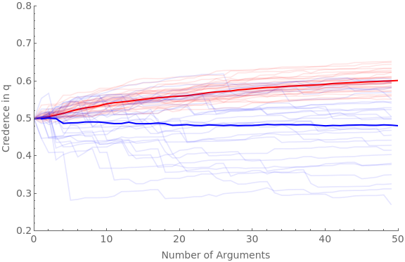
Given these two functions, we can simulate presenting a group of (red) agents with random arguments that favor q, and a separate group of (blue) agents with random arguments that disfavor q.
numAgents = the number of agents in each group
numArgs = the number of arguments each agent sees
baseShift = the base constraint on how far arguments could in principle move opinions; range between 0–0.5. (Depending on hardenSpeed, the amount of shift may be less extreme than its raw number)
hardenSpeed = how quickly the shift induced by each argument tapers off. Recommended between 0.2–0.5
In[]:=
Clear[ag];Clear[traj];numAgents=20;numArgs=100;baseShift=0.4;hardenSpeed=0.2;(*hardening=True;If[hardeningTrue,harden[x_]:=Sqrt[x]]If[hardeningFalse,harden[x_]:=1]*)simTime=Timing[Do[If[valence"pro",Do[iter1;ticker=10;ag[cred,iter1,valence]=0.5;ag[traj,iter1,valence]=Reap[Do[priorG=RandomReal[{0,1}];Sow[{ticker-10,ag[cred,iter1,valence]}];frame=getRandFavShiftArgModel[ag[cred,iter1,valence],baseShift/(hardenSpeed*ticker),priorG];If[RandomVariate[BernoulliDistribution[priorG]]1,postFxn=frame[[2]],postFxn=frame[[4]]];ag[cred,iter1,valence]=probability[postFxn,{2,4}];ticker+=1;,numArgs]][[2,1]];,{iter1,numAgents}]];If[valence"con",Do[iter1;ticker=10;ag[cred,iter1,valence]=0.5;ag[traj,iter1,valence]=Reap[Do[priorG=RandomReal[{0,1}];Sow[{ticker-10,ag[cred,iter1,valence]}];frame=getRandDisShiftArgModel[ag[cred,iter1,valence],baseShift/(hardenSpeed*ticker),priorG];If[RandomVariate[BernoulliDistribution[priorG]]1,postFxn=frame[[2]],postFxn=frame[[4]]];ag[cred,iter1,valence]=probability[postFxn,{2,4}];ticker+=1;,numArgs]][[2,1]];,{iter1,numAgents}]];,{valence,{"pro","con"}}]][[1]];Beep[]Clear[allAgents];allAgents["pro"]=ag[traj,#,"pro"]&/@Range[numAgents];allAgents["con"]=ag[traj,#,"con"]&/@Range[numAgents];avgAgents["pro"]=Table[{iter1,Mean[ag[traj,#,"pro"][[iter1,2]]&/@Range[numAgents]]},{iter1,numArgs}];avgAgents["con"]=Table[{iter1,Mean[ag[traj,#,"con"][[iter1,2]]&/@Range[numAgents]]},{iter1,numArgs}];Show[ListLinePlot[allAgents["pro"],PlotStyleDirective[Red,Opacity[0.1]],PlotRange{{0,numArgs},{0.2,0.8}},Frame{{True,False},{True,False}},ImageSizeLarge,FrameLabel{{Style["Credence in q",FontSize14],None},{Style["Number of Arguments",FontSize14],None}},FrameTicksAll,FrameTicksStyleDirective[FontSize14]],ListLinePlot[avgAgents["pro"],PlotStyleDirective[Red,Thick]],ListLinePlot[allAgents["con"],PlotStyleDirective[Blue,Opacity[0.1]]],ListLinePlot[avgAgents["con"],PlotStyleDirective[Blue,Thick]]]Print[StringForm["Simulation time = ``",simTime]]
Out[]=
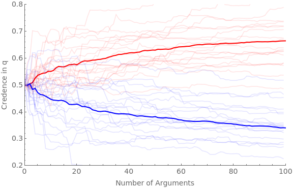
Simulation time = 50.6017
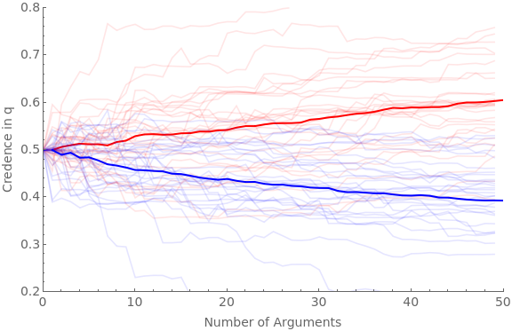
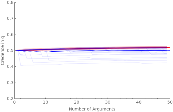
The following simulation lets you vary what proportion of the arguments are good. Whereas the above pulled π(G) randomly between [0,1] for both sides, this one pulls π(G) from [favGBound,1] for the “pro” side, and π(G) from [0, 1–favGBound] for the “con” side.
The following code runs the simulation for 30 agents and 50 arguments with favGBound at 0, 0.25, 0.5, 0.75, and 0.95:
The following code runs the simulation for 30 agents and 50 arguments with favGBound at 0, 0.25, 0.5, 0.75, and 0.95:
numAgents=30;numArgs=50;Do[favGBound=boundIter;Clear[ag];Clear[traj];baseShift=0.4;hardenSpeed=0.2;(*hardening=True;If[hardeningTrue,harden[x_]:=Sqrt[x]]If[hardeningFalse,harden[x_]:=1]*)simTime=Timing[Do[If[valence"pro",Do[iter1;ticker=10;ag[cred,iter1,valence]=0.5;ag[traj,iter1,valence]=Reap[Do[priorG=RandomReal[{favGBound,1}];Sow[{ticker-10,ag[cred,iter1,valence]}];frame=getRandFavShiftArgModel[ag[cred,iter1,valence],baseShift/(hardenSpeed*ticker),priorG];If[RandomVariate[BernoulliDistribution[priorG]]1,postFxn=frame[[2]],postFxn=frame[[4]]];ag[cred,iter1,valence]=probability[postFxn,{2,4}];ticker+=1;,numArgs]][[2,1]];,{iter1,numAgents}]];If[valence"con",Do[iter1;ticker=10;ag[cred,iter1,valence]=0.5;ag[traj,iter1,valence]=Reap[Do[priorG=RandomReal[{0,1-favGBound}];Sow[{ticker-10,ag[cred,iter1,valence]}];frame=getRandDisShiftArgModel[ag[cred,iter1,valence],baseShift/(hardenSpeed*ticker),priorG];If[RandomVariate[BernoulliDistribution[priorG]]1,postFxn=frame[[2]],postFxn=frame[[4]]];ag[cred,iter1,valence]=probability[postFxn,{2,4}];ticker+=1;,numArgs]][[2,1]];,{iter1,numAgents}]];,{valence,{"pro","con"}}]][[1]];Beep[];Clear[allAgents];allAgents["pro"]=ag[traj,#,"pro"]&/@Range[numAgents];allAgents["con"]=ag[traj,#,"con"]&/@Range[numAgents];avgAgents["pro"]=Table[{iter1,Mean[ag[traj,#,"pro"][[iter1,2]]&/@Range[numAgents]]},{iter1,numArgs}];avgAgents["con"]=Table[{iter1,Mean[ag[traj,#,"con"][[iter1,2]]&/@Range[numAgents]]},{iter1,numArgs}];Print[StringForm["Simulation time = ``, favGBound = ``",simTime,favGBound]];Print[Show[ListLinePlot[allAgents["pro"],PlotStyleDirective[Red,Opacity[0.1]],PlotRange{{0,numArgs},{0.2,0.8}},Frame{{True,False},{True,False}},ImageSizeLarge,FrameLabel{{Style["Credence in q",FontSize14],None},{Style["Number of Arguments",FontSize14],None}},FrameTicksAll,FrameTicksStyleDirective[FontSize14]],ListLinePlot[avgAgents["pro"],PlotStyleDirective[Red,Thick]],ListLinePlot[allAgents["con"],PlotStyleDirective[Blue,Opacity[0.1]]],ListLinePlot[avgAgents["con"],PlotStyleDirective[Blue,Thick]]]];,{boundIter,{0,0.25,0.5,0.75,0.95}}]
Simulation time = 44.7012, favGBound = 0
Simulation time = 42.0477, favGBound = 0.25
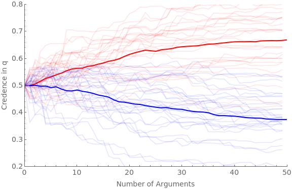
Simulation time = 38.1415, favGBound = 0.5
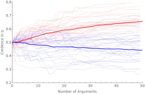
Simulation time = 40.718, favGBound = 0.75
Simulation time = 42.6826, favGBound = 0.95
Robustness
Robustness
(3) Combined Model
(3) Combined Model
The extractArgPars takes an argument model and extracts the parameters needed to generate it, and loads them into the variable-names as specified in the commented section:
In[]:=
(*requiresa(5-world)argmodel*)extractArgPars[frame_]:=((*loadsup:priorQ=priorinqbeforeargumentgInf=informedcredenceinqwhenargumentgoodbInf=informedcredenceinqwhenargumentbadpriorG=priorcredencethatargumentgoodpriorB=priorcreencethatargumentbadbConf=posteriorconfidencethatargumentbad(ifitis)gConf=posteriorconfidencethatargumentgood(ifitis)*)priorQ=probability[frame[[1]],{2,4}];gInf=frame[[2,2]]/(frame[[2,2]]+frame[[2,3]]);bInf=frame[[4,4]]/(frame[[4,4]]+frame[[4,5]]);(*priorG=x/.Solve[priorQx*(gInf)+(1-x)(bInf),x][[1]];*)priorG=probability[frame[[1]],{2,3}];priorB=1-priorG;bConf=(1-x)/.Solve[probability[frame[[4]],{2,4}]x*gInf+(1-x)(bInf),x][[1]];gConf=x/.Solve[probability[frame[[2]],{2,4}]x*gInf+(1-x)(bInf),x][[1]];)
For example, if we get a random argument, we can extract it’s parameters and remake it:
In[]:=
frame=getRandFavShiftArgModel[0.5,0.2,0.5]
Out[]=
{{0,0.261666,0.238334,0.238334,0.261666},{0,0.460661,0.419585,0.0570828,0.0626711},{0,0.460661,0.419585,0.0570828,0.0626711},{0,0.256276,0.233424,0.243243,0.267056},{0,0.256276,0.233424,0.243243,0.267056}}
In[]:=
extractArgPars[frame]
In[]:=
getArgModel[priorQ,gInf,gConf,bInf,bConf]
Out[]=
{{0,0.261666,0.238334,0.238334,0.261666},{0,0.460661,0.419585,0.0570828,0.0626711},{0,0.460661,0.419585,0.0570828,0.0626711},{0,0.256276,0.233424,0.243243,0.267056},{0,0.256276,0.233424,0.243243,0.267056}}
The scrutArg function takes an argument model (frame), a probability of finding a flaw if there is one (pFind), and a degree to which scrutiny increases ambiguity (jShift), and outputs a cognitive search model that results from scrutinizing it, meeting the relevant parameters as specified in Appendix C.3:
In[]:=
(*generatescrutinymodelbasedonargumentmodelsuchthatifargumentisgood,conditiononnot-findingaproblem(word);andifargumentbadbutdon'tfind,J-shiftuponthatfact*)(*J-shiftaparameterbetween0and1sayinghowmuchposteriorconfinNfW(possibilitywherethere'sacompletionyoudon'tfind)movestoward1fromthebaselineofsimplyconditioningonNf*)scrutArg[frame_,pFind_,jShift_]:=(extractArgPars[frame];(*loadsup:priorQ=priorinqbeforeargumentgInf=informedcredenceinqwhenargumentgoodbInf=informedcredenceinqwhenargumentbadpriorG=priorcredencethatargumentgoodpriorB=priorcreencethatargumentbadbConf=posteriorconfidencethatargumentbad(ifitis)gConf=posteriorconfidencethatargumentgood(ifitis)*)(*informedprobabilityifwordisbInf,sobumpis:*)wBump=bInf-priorQ;priorFW=priorB*pFind;priorNfW=priorB*(1-pFind);priorNfNw=priorG;(*posteriorconfidencethatnowordobtainedbyconditioningonnofind*)postNwConf=gConf/(gConf+(1-gConf)(1-pFind));(*posteriorconfinNfWifjustconditionedonNf:*)NfWCond=(bConf(1-pFind))/(bConf(1-pFind)+(1-bConf));(*Howmuchshouldyourconfidencethatthere'sawordshifttowardtherebeingoneifthereisonethatyoudon'tfind?*)postNfWConf=(1-jShift)*NfWCond+jShift*1;Return[csQModel[priorQ,wBump,priorFW,priorNfW,priorNfNw,postNfWConf,postNwConf]])
For example, here’s our above randomly-generated argument model, along with what happens when we scrutinize it:
In[]:=
MatrixForm[frame]MatrixForm[scrutArg[frame,0.5,0.5]]
Out[]//MatrixForm=
0 | 0.261666 | 0.238334 | 0.238334 | 0.261666 |
0 | 0.460661 | 0.419585 | 0.0570828 | 0.0626711 |
0 | 0.460661 | 0.419585 | 0.0570828 | 0.0626711 |
0 | 0.256276 | 0.233424 | 0.243243 | 0.267056 |
0 | 0.256276 | 0.233424 | 0.243243 | 0.267056 |
Out[]//MatrixForm=
0 | 0.261666 | 0.238334 | 0.119167 | 0.130833 | 0.119167 | 0.130833 |
0 | 0.490001 | 0.446308 | 0.0303592 | 0.0333313 | 0 | 0 |
0 | 0.490001 | 0.446308 | 0.0303592 | 0.0333313 | 0 | 0 |
0 | 0.172032 | 0.156692 | 0.319976 | 0.3513 | 0 | 0 |
0 | 0.172032 | 0.156692 | 0.319976 | 0.3513 | 0 | 0 |
0 | 0 | 0 | 0 | 0 | 0.476668 | 0.523332 |
0 | 0 | 0 | 0 | 0 | 0.476668 | 0.523332 |
Notice a few things about this model of scrutinizing arguments.
First, when you are guaranteed to find a flaw if there is one (π(Find | Flaw) = pFind = 1), then regardless of the jShift parameter, scrutiny turns the ambiguous-evidence argument into an unambiguous update (although the possibilities in C, i.e. 4 and 5, differ from those in N, i.e. 2 and 3, the prior and N assign probability 0 to these possibilities):
First, when you are guaranteed to find a flaw if there is one (π(Find | Flaw) = pFind = 1), then regardless of the jShift parameter, scrutiny turns the ambiguous-evidence argument into an unambiguous update (although the possibilities in C, i.e. 4 and 5, differ from those in N, i.e. 2 and 3, the prior and N assign probability 0 to these possibilities):
In[]:=
MatrixForm[frame=getRandFavShiftArgModel[0.5,0.2,0.5]]MatrixForm[scrutArg[frame,1,0.5]]
Out[]//MatrixForm=
0 | 0.325654 | 0.174346 | 0.174346 | 0.325654 |
0 | 0.432748 | 0.23168 | 0.117011 | 0.218561 |
0 | 0.432748 | 0.23168 | 0.117011 | 0.218561 |
0 | 0.228577 | 0.122373 | 0.226318 | 0.422732 |
0 | 0.228577 | 0.122373 | 0.226318 | 0.422732 |
Out[]//MatrixForm=
0 | 0.325654 | 0.174346 | 0. | 0. | 0.174346 | 0.325654 |
0 | 0.651309 | 0.348691 | 0. | 0. | 0 | 0 |
0 | 0.651309 | 0.348691 | 0. | 0. | 0 | 0 |
0 | 0.325654 | 0.174346 | 0.174346 | 0.325654 | 0 | 0 |
0 | 0.325654 | 0.174346 | 0.174346 | 0.325654 | 0 | 0 |
0 | 0 | 0 | 0 | 0 | 0.348691 | 0.651309 |
0 | 0 | 0 | 0 | 0 | 0.348691 | 0.651309 |
Second, if you are guaranteed not to find a flaw in the argument if there is one (you know it’s to complex), then---at least with the further plausible assumption that scrutiny adds no ambiguity (you don’t think “maybe I should’ve found it)---then scrutiny leaves the initial argument model unchanged (there is no possibility of ending up in F = {6,7}):
In[]:=
MatrixForm[frame=getRandFavShiftArgModel[0.5,0.2,0.5]]MatrixForm[scrutArg[frame,0,0]]
Out[]//MatrixForm=
0 | 0.27327 | 0.22673 | 0.22673 | 0.27327 |
0 | 0.321346 | 0.266617 | 0.186842 | 0.225195 |
0 | 0.321346 | 0.266617 | 0.186842 | 0.225195 |
0 | 0.243994 | 0.202439 | 0.25102 | 0.302547 |
0 | 0.243994 | 0.202439 | 0.25102 | 0.302547 |
Out[]//MatrixForm=
0 | 0.27327 | 0.22673 | 0.22673 | 0.27327 | 0. | 0. |
0 | 0.321346 | 0.266617 | 0.186842 | 0.225195 | 0 | 0 |
0 | 0.321346 | 0.266617 | 0.186842 | 0.225195 | 0 | 0 |
0 | 0.243994 | 0.202439 | 0.25102 | 0.302547 | 0 | 0 |
0 | 0.243994 | 0.202439 | 0.25102 | 0.302547 | 0 | 0 |
0 | 0 | 0 | 0 | 0 | 0.453459 | 0.546541 |
0 | 0 | 0 | 0 | 0 | 0.453459 | 0.546541 |
Finally, for values between these extremes, scrutiny makes some difference:
In[]:=
MatrixForm[frame=getRandFavShiftArgModel[0.5,0.2,0.5]]MatrixForm[scrutArg[frame,0.5,0.5]]
Out[]//MatrixForm=
0 | 0.287695 | 0.212305 | 0.212305 | 0.287695 |
0 | 0.434301 | 0.320494 | 0.104116 | 0.141088 |
0 | 0.434301 | 0.320494 | 0.104116 | 0.141088 |
0 | 0.253608 | 0.187151 | 0.23746 | 0.321782 |
0 | 0.253608 | 0.187151 | 0.23746 | 0.321782 |
Out[]//MatrixForm=
0 | 0.287695 | 0.212305 | 0.106153 | 0.143847 | 0.106153 | 0.143847 |
0 | 0.494988 | 0.365278 | 0.0593325 | 0.0804015 | 0 | 0 |
0 | 0.494988 | 0.365278 | 0.0593325 | 0.0804015 | 0 | 0 |
0 | 0.176024 | 0.129897 | 0.294713 | 0.399366 | 0 | 0 |
0 | 0.176024 | 0.129897 | 0.294713 | 0.399366 | 0 | 0 |
0 | 0 | 0 | 0 | 0 | 0.424611 | 0.575389 |
0 | 0 | 0 | 0 | 0 | 0.424611 | 0.575389 |
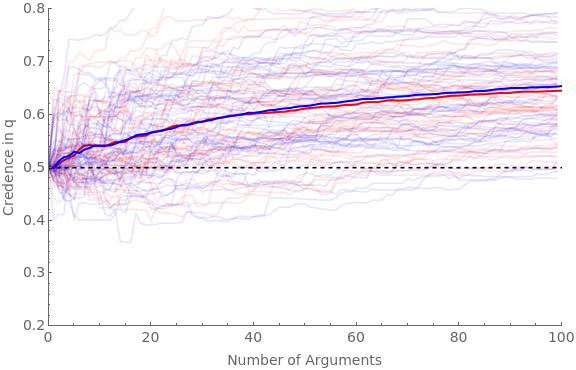
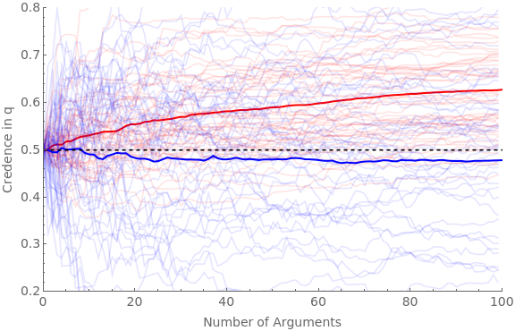
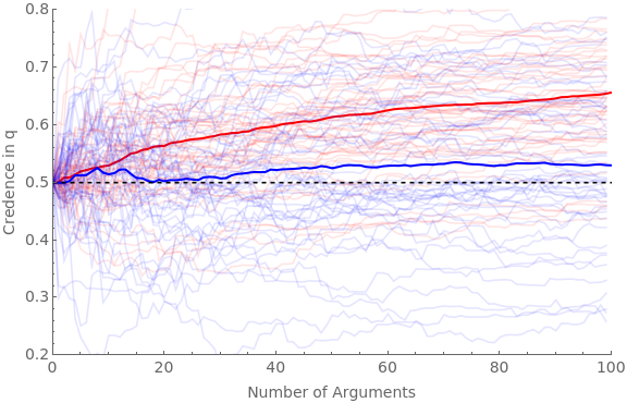
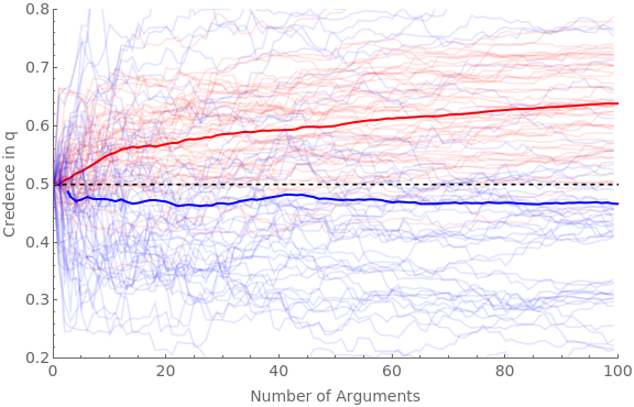
We can now simulate what happens when both pro (red) and con (blue) agents are presented with favorable arguments (with the same parameters as the main simulation in section 2 above), but where red never scrutinizes them and blue always does.
We will run four versions: (1) where blue agents NEVER find flaws in the argument if there are any; (2) where they ALWAYS do; (3) where they sometimes do, and scrutiny adds a small amount of ambiguity; and (4) where they sometimes do, and scrutiny adds a middling amount of ambiguity.
We will run four versions: (1) where blue agents NEVER find flaws in the argument if there are any; (2) where they ALWAYS do; (3) where they sometimes do, and scrutiny adds a small amount of ambiguity; and (4) where they sometimes do, and scrutiny adds a middling amount of ambiguity.
In[]:=
Clear[ag];Clear[traj];numAgents=50;numArgs=100;baseShift=0.4;hardenSpeed=0.2;Do[pFindIter=iter[[1]];jShiftIter=iter[[2]];pFindBnds={pFindIter[[1]],pFindIter[[2]]};jShiftBnds={jShiftIter[[1]],jShiftIter[[2]]};simTime=Timing[Do[(*proagentsNEVERscrutinize*)If[valence"pro",Do[iter1;ticker=10;ag[cred,iter1,valence]=0.5;ag[traj,iter1,valence]=Reap[Do[(*getanargumentmodel:*)priorG=RandomReal[{0,1}];Sow[{ticker-10,ag[cred,iter1,valence]}];frame=getRandFavShiftArgModel[ag[cred,iter1,valence],baseShift/(hardenSpeed*ticker),priorG];(*updatebeliefs:*)If[RandomVariate[BernoulliDistribution[priorG]]1,postFxn=frame[[2]],postFxn=frame[[4]]];ag[cred,iter1,valence]=probability[postFxn,{2,4}];ticker+=1;,numArgs]][[2,1]];,{iter1,numAgents}]];(*conagentsALWAYSscrutinize:*)If[valence"con",Do[iter1;ticker=10;ag[cred,iter1,valence]=0.5;ag[traj,iter1,valence]=Reap[Do[(*getafavorableargumentmodel*)priorG=RandomReal[{0,1}];Sow[{ticker-10,ag[cred,iter1,valence]}];frame=getRandFavShiftArgModel[ag[cred,iter1,valence],baseShift/(hardenSpeed*ticker),priorG];(*makethescrutinizedmodel:*)pFind=RandomReal[{pFindBnds[[1]],pFindBnds[[2]]}];jShift=RandomReal[{jShiftBnds[[1]],jShiftBnds[[2]]}];scrutFrame=scrutArg[frame,pFind,jShift];(*updatebeliefsviascrutinizedmodel:*)If[RandomVariate[BernoulliDistribution[priorG]]1,postFxn=scrutFrame[[2]],If[RandomVariate[BernoulliDistribution[pFind]]1,postFxn=scrutFrame[[6]],postFxn=scrutFrame[[4]]]];ag[cred,iter1,valence]=probability[postFxn,{2,4,6}];ticker+=1;,numArgs]][[2,1]];,{iter1,numAgents}]];,{valence,{"pro","con"}}]][[1]];Beep[];Clear[allAgents];allAgents["pro"]=ag[traj,#,"pro"]&/@Range[numAgents];allAgents["con"]=ag[traj,#,"con"]&/@Range[numAgents];avgAgents["pro"]=Table[{iter1,Mean[ag[traj,#,"pro"][[iter1,2]]&/@Range[numAgents]]},{iter1,numArgs}];avgAgents["con"]=Table[{iter1,Mean[ag[traj,#,"con"][[iter1,2]]&/@Range[numAgents]]},{iter1,numArgs}];Print[StringForm["Simulation time = ``, pFind bounds = ``, jShift bounds = ``",simTime,pFindBnds,jShiftBnds]];Print[Show[ListLinePlot[allAgents["pro"],PlotStyleDirective[Red,Opacity[0.1]],PlotRange{{0,numArgs},{0.2,0.8}},Frame{{True,False},{True,False}},ImageSizeLarge,FrameLabel{{Style["Credence in q",FontSize14],None},{Style["Number of Arguments",FontSize14],None}},FrameTicksAll,FrameTicksStyleDirective[FontSize14]],ListLinePlot[avgAgents["pro"],PlotStyleDirective[Red,Thick]],ListLinePlot[allAgents["con"],PlotStyleDirective[Blue,Opacity[0.1]]],ListLinePlot[avgAgents["con"],PlotStyleDirective[Blue,Thick]],Plot[0.5,{x,0,numArgs},PlotStyle{Black,Dashed}]]];,{iter,(*firstpairispFindBnds,secondisjShiftBnds*){{{0,0},{0,0}},(*neverfind,noaddedambiguity*){{1,1},{0,1}},(*alwaysfind,randomaddedambiguity*){{0,1},{0,0.5}},(*randomprobabilityoffind;addlittleambiguity*){{0,1},{0,1}}(*randomprobabilityoffind,addrandomambiguity*)}}]
Simulation time = 139.714, pFind bounds = {0,0}, jShift bounds = {0,0}
Simulation time = 129.31, pFind bounds = {1,1}, jShift bounds = {0,1}
Simulation time = 138.604, pFind bounds = {0,1}, jShift bounds = {0,0.5}
Simulation time = 146.383, pFind bounds = {0,1}, jShift bounds = {0,1}
Robustness
Robustness