ABSTRACT (original article): OpenAI’s reasoning model o3-mini-high was used to carry out an exact analytic study of one-dimensional ferrimagnetic decorated -state Potts models. We demonstrate that the finite-temperature ultranarrow phase crossover (UNPC), driven by a hidden “half-ice, half-fire” state in the Potts (Ising) model, persists for . We identify novel features for , including the dome structure in the field-temperature phase diagram and for large a secondary high-temperature UNPC to the fully disordered paramagnetic state. The ice-fire mechanism of spin flipping can be applied to higher-dimensional Potts models. These results establish a versatile framework for engineering controlled fast state-flipping switches in low-dimensional systems. Our nine-level AI-contribution rating assigns AI the meritorious status of AI-co-led discovery in this work. CITATION (original article): Weiguo Yin (2025), Half-Ice, Half-Fire Driven Ultranarrow Phase Crossover in 1D Decorated q-State Potts Ferrimagnets: An AI-Co-Led Discovery, arXiv:2505.02303. https://doi.org/10.48550/arXiv.2505.02303
q
q=2
q>2
q>2
q
Introduction
Introduction
The -state Potts model is a fundamental theoretical framework for understanding exotic phases and phase transitions, with applications spanning from magnetic materials to protein sequence analysis. However, one-dimensional (1D) Potts models with short-range interactions are well-known to lack finite-temperature phase transitions; hence, they have been largely overlooked for their potentials in technological applications. Recently, a finite-temperature ultranarrow phase crossover (UNPC), driven by a previously hidden “half-ice, half-fire” state, was discovered in 1D decorated Potts models for the simplest case (, known as the Ising model). Here, leveraging OpenAI’s advanced reasoning model o3-mini-high, we rigorously show that this half-ice, half-fire driven UNPC robustly persists for all , exhibiting remarkable new features such as a dome-shaped structure in the field-temperature phase diagram and, for large q, an additional high-temperature UNPC transitioning into the fully disordered paramagnetic state. Our findings establish a versatile theoretical platform for designing rapid, controlled phase switching in low-dimensional materials, and demonstrate the unprecedented capability of AI to assimilate novel theoretical concepts and immediately apply them toward pioneering frontier research, culminating in authentic scientific discoveries. Wolfram Mathematica was used to verify the symbolic derivations of the human and AI researchers such as the equivalence of different theoretical approaches and vividly display the results as a melody of ice and fire.
q
q2
q>2
AI Contribution
AI Contribution
o3-mini-high was asked to read two recent papers (arXiv:2502.11270 and arXiv:2503.23758) and suggest future work. The AI pointed out five directions with the first one being the present study. Then, it integrated the models and algorithms in the two papers to carry out all the setup, derivation, coding, and drafting the math-heavy technical sections with minimal human interference in a few minutes---most insightfully it predicted exactly how to identify UNPCs and the half ice, half-fire mechanism for arbitrary ---thus earning its meritorious AI-co-led status (see End Matter B for details).
q
Critical Human-AI Interaction
Critical Human-AI Interaction
The AI tried directly using the MSS method (arXiv:2503.23758) to reduce the transfer matrix to the maximally symmetric subspace but it quickly realized that this only worked for . The human researcher reminded the AI that the decoration part can be exactly summed out. Then the AI used the method (arXiv:2502.11270) to exactly sum out the decorating spins and the MSS method to reduce the resulting transfer matrix to .
2
q
2
q
22
h0
qq
22
Model and Mapping
Model and Mapping
Kronecker delta
In[]:=
ClearAll[tol,delta,Ndelta];delta[x_,y_]:=If[x===y,1,0];tol=1.*10^(-5);Ndelta[x_,y_]:=If[x>1/tol,Abs[y/x-1.]<tol,Abs[y-x]<tol];
Standard Potts model in a magnetic field without decoration . It is used to test the limiting case and the effective magnetic field method
Build the q x q transfer matrix TmatB
In[]:=
ClearAll[x,B,q,TMatB];(*x,B*)TMatB[x_,B_,q_]:=Table[Module[{bondTerm,fieldTerm},bondTerm=x^delta[i,j];fieldTerm=B^(delta[i,1]+delta[j,1]);bondTerm*fieldTerm],{i,1,q},{j,1,q}];{TMatB[x,B,3]//MatrixForm,TMatB[x,B,4]//MatrixForm,TMatB[x,B,5]//MatrixForm}
βJ
e
βh2
μ
a
e
Out[]=
,
,
2 B | B | B |
B | x | 1 |
B | 1 | x |
2 B | B | B | B |
B | x | 1 | 1 |
B | 1 | x | 1 |
B | 1 | 1 | x |
2 B | B | B | B | B |
B | x | 1 | 1 | 1 |
B | 1 | x | 1 | 1 |
B | 1 | 1 | x | 1 |
B | 1 | 1 | 1 | x |
1. Build the q x q transfer matrix TMatrix with the decorating spins being summed out
In[]:=
Clear[x,y,a,b,q,TMatrix](*x,y,a,b*)TMatrix[x_,a_,y_,b_,q_]:=Table[Module[{bondTerm,fieldTerm,decorated},bondTerm=x^delta[i,j];fieldTerm=a^(delta[i,1]+delta[j,1]);decorated=0;Do[decorated=decorated+b^(delta[i1,1]+delta[j1,1])*y^(delta[i1,i]+delta[j1,j]),{i1,1,q},{j1,1,q}];decorated=Simplify[Sqrt[Factor[decorated]],b>0&&y>0];bondTerm*fieldTerm*decorated],{i,1,q},{j,1,q}];Print["TMatrix[x,a,y,b,q=3]= ",TMatrix[x,a,y,b,3]//MatrixForm];Print[">>>>>Checkpoint 1: 0,0 (i.e., y=1, b=1)"];Print[" TMatrix[x,a,1,1,q=3]= ",TMatrix[x,a,1,1,3]//MatrixForm];Do[Print[" TMatrix[x,a,1,1,q]===TMatB[x,a,q] * q (q=",q,")? ",TMatrix[x,a,1,1,q]===TMatB[x,a,q]*q],{q,2,5}];Print[">>>>>Checkpoint 2: 0,≠0 (i.e., y=1)"];Print[" TMatrix[x,a,1,b,q=3]= ",TMatrix[x,a,1,b,3]//MatrixForm];Do[Print[" TMatrix[x,a,1,b,q]===TMatB[x,a,q] * (b+q-1) (q=",q,")? ",TMatrix[x,a,1,b,q]===TMatB[x,a,q]*(b+q-1)],{q,2,5}]
βJ
e
β
J
ab
e
βh2
μ
a
e
βh
μ
b
e
J
ab
μ
b
J
ab
μ
b
TMatrix[x,a,y,b,q=3]=
2 a | a (1+b+y)(2+by) | a (1+b+y)(2+by) |
a (1+b+y)(2+by) | x(1+b+y) | 1+b+y |
a (1+b+y)(2+by) | 1+b+y | x(1+b+y) |
>>>>>Checkpoint 1: 0,0 (i.e., y=1, b=1)
J
ab
μ
b
TMatrix[x,a,1,1,q=3]=
3 2 a | 3a | 3a |
3a | 3x | 3 |
3a | 3 | 3x |
TMatrix[x,a,1,1,q]===TMatB[x,a,q] * q (q=2)? True
TMatrix[x,a,1,1,q]===TMatB[x,a,q] * q (q=3)? True
TMatrix[x,a,1,1,q]===TMatB[x,a,q] * q (q=4)? True
TMatrix[x,a,1,1,q]===TMatB[x,a,q] * q (q=5)? True
>>>>>Checkpoint 2: 0,≠0 (i.e., y=1)
J
ab
μ
b
TMatrix[x,a,1,b,q=3]=
2 a | a(2+b) | a(2+b) |
a(2+b) | (2+b)x | 2+b |
a(2+b) | 2+b | (2+b)x |
TMatrix[x,a,1,b,q]===TMatB[x,a,q] * (b+q-1) (q=2)? True
TMatrix[x,a,1,b,q]===TMatB[x,a,q] * (b+q-1) (q=3)? True
TMatrix[x,a,1,b,q]===TMatB[x,a,q] * (b+q-1) (q=4)? True
TMatrix[x,a,1,b,q]===TMatB[x,a,q] * (b+q-1) (q=5)? True
Mapping onto an effective magnetic field, see Equations (4) - (8)
In[]:=
Clear[TMatBeff,aeff](*x,y,a,b*)aeff[a_,b_,y_,q_]:=aSqrt[(by+q-1)/(b+y+q-2)];TMatBeff[x_,a_,y_,b_,q_]:=PowerExpand[TMatB[x,aeff[a,b,y,q],q]*(b+y+q-2)]//.Power[s_,m_]Power[t_,m_]:>Power[st,m];Print["The effective field method:"];Do[Print["TMatBeff[x,a,y,b,q] (q=",q,")= ",TMatBeff[x,a,y,b,q]//MatrixForm],{q,3,3}];Print[">>>>>Checkpoint 3: Must agree with the previous method"];Do[Print[" TMatrix[x,a,y,b,q]===TMatBeff[x,a,y,b,q] (q=",q,")? ",TMatrix[x,a,y,b,q]===TMatBeff[x,a,y,b,q]],{q,2,5}];
βJ
e
β
J
ab
e
βh2
μ
a
e
βh
μ
b
e
The effective field method:
TMatBeff[x,a,y,b,q] (q=3)=
2 a | a (1+b+y)(2+by) | a (1+b+y)(2+by) |
a (1+b+y)(2+by) | x(1+b+y) | 1+b+y |
a (1+b+y)(2+by) | 1+b+y | x(1+b+y) |
>>>>>Checkpoint 3: Must agree with the previous method
TMatrix[x,a,y,b,q]===TMatBeff[x,a,y,b,q] (q=2)? True
TMatrix[x,a,y,b,q]===TMatBeff[x,a,y,b,q] (q=3)? True
TMatrix[x,a,y,b,q]===TMatBeff[x,a,y,b,q] (q=4)? True
TMatrix[x,a,y,b,q]===TMatBeff[x,a,y,b,q] (q=5)? True
2. Using the MSS method to reduce the transfer matrix to the 2 x2 maximally symmetric subspace : Equations (9) and (10)
In[]:=
Clear[Tblock22,Tblock22eff](*x,y,a,b*)Tblock22[x_,a_,y_,b_,q_]:=Module[{e1,e2,V2q,Vq2},(*Create2MSSbasisvectors*)e1=Normalize[Table[If[i==1,1,0],{i,1,q}]];e2=Normalize[Table[If[i!=1,1,0],{i,1,q}]];V2q={e1,e2};Vq2=Transpose[V2q];If[q<=5,Print["MSS basis:\n",V2q//MatrixForm]];FullSimplify[V2q.TMatrix[x,a,y,b,q].Vq2]]Do[Print["Tblock22[x,a,y,b,q] (q=",q,")= ",Tblock22[x,a,y,b,q]//MatrixForm],{q,3,3}];(*Theeffectivefieldmethod*)Tblock22eff[x_,a_,y_,b_,q_]:=Module[{e1,e2,V2q,Vq2},(*Create2MSSbasisvectors*)e1=Normalize[Table[If[i==1,1,0],{i,1,q}]];e2=Normalize[Table[If[i!=1,1,0],{i,1,q}]];V2q={e1,e2};Vq2=Transpose[V2q];(*If[q<=5,Print["MSS basis for the effective field method:\n",V2q//MatrixForm]];*)FullSimplify[V2q.TMatBeff[x,a,b,y,q].Vq2]]Do[Print["Tblock22eff[x,a,y,b,q] (q=",q,")= ",Tblock22eff[x,a,y,b,q]//MatrixForm],{q,3,3}];Print[">>>>>Checkpoint 4: Must agree with the previous method"];Do[Print[" Tblock22[x,a,y,b,q]===Tblock22eff[x,a,y,b,q] (q=",q,")? ",Tblock22[x,a,y,b,q]===Tblock22eff[x,a,y,b,q]],{q,2,5}];
βJ
e
β
J
ab
e
βh2
μ
a
e
βh
μ
b
e
MSS basis:
1 | 0 | 0 |
0 | 1 2 | 1 2 |
Tblock22[x,a,y,b,q] (q=3)=
2 a | 2 a(1+b+y)(2+by) |
2 a(1+b+y)(2+by) | (1+x)(1+b+y) |
Tblock22eff[x,a,y,b,q] (q=3)=
2 a | 2 a(1+b+y)(2+by) |
2 a(1+b+y)(2+by) | (1+x)(1+b+y) |
>>>>>Checkpoint 4: Must agree with the previous method
MSS basis:
1 | 0 |
0 | 1 |
Tblock22[x,a,y,b,q]===Tblock22eff[x,a,y,b,q] (q=2)? True
MSS basis:
1 | 0 | 0 |
0 | 1 2 | 1 2 |
Tblock22[x,a,y,b,q]===Tblock22eff[x,a,y,b,q] (q=3)? True
MSS basis:
1 | 0 | 0 | 0 |
0 | 1 3 | 1 3 | 1 3 |
Tblock22[x,a,y,b,q]===Tblock22eff[x,a,y,b,q] (q=4)? True
MSS basis:
1 | 0 | 0 | 0 | 0 |
0 | 1 2 | 1 2 | 1 2 | 1 2 |
Tblock22[x,a,y,b,q]===Tblock22eff[x,a,y,b,q] (q=5)? True
3. The largest eigenvalue of the transfer matrix : Equation (11)
In[]:=
Clear[lambda,lambdaEff]lambda[t_,h_,J_,mua_,Jb_,mub_,q_]:=Module{u,v,w,x,y,a,b},(*x,y,a,b*)x=Exp[J/t];y=Exp[Jb/t];a=Exp[0.5hmua/t];b=Exp[hmub/t];u=a^2x(q-1+by);v=(x+q-2)(q-2+b+y);w=Sqrt[q-1]aSqrt[(q-1+by)(q-2+b+y)];(u+v)2+Sqrt[((u-v)/2)^2+w^2]lambdaEff[t_,h_,J_,mua_,Jb_,mub_,q_]:=Module{u,v,w,x,y,a,b,CF,aeff0},(*x,y,a,b*)x=Exp[J/t];y=Exp[Jb/t];a=Exp[0.5hmua/t];b=Exp[hmub/t];CF=q-2+b+y;aeff0=aSqrt[(q-1+by)/(q-2+b+y)];u=CFaeff0^2x;v=CF(x+q-2);w=CFSqrt[q-1]aeff0;(u+v)2+Sqrt[((u-v)/2)^2+w^2](*NumericalTest*)Clear[para,para0,q,x,y,a,b,t,h,J,Jb,mua,mub,lmda,eigs0,eigs2,eigv0];q=3para={t->1.,h->1.5,J->1.,Jb->-1.,mua->1.,mub->4./3};para0={x->Exp[J/t],y->Exp[Jb/t],a->Exp[0.5hmua/t],b->Exp[hmub/t]}/.paralmda=Chop[lambda[t,h,J,mua,Jb,mub,q]/.para]lmdaEff=Chop[lambdaEff[t,h,J,mua,Jb,mub,q]/.para]eigs0=Chop[Eigenvalues[TMatrix[x,a,y,b,q]/.para0]];If[q<=5,Print["Eigenvalues of TMatrix: ",eigs0]];Print["The largest eigenvalues of TMatrix : ",eigs0[[1]]];Print["The second largest eigenvalues of TMatrix : ",eigs0[[2]]];Print["The smallest eigenvalues of TMatrix : ",eigs0[[q]]];If[q<=5,{eigs0,eigv0}=Eigensystem[TMatrix[x,a,y,b,q]/.para0];Print["Eigenvectors: ",Transpose[Chop[eigv0]]//MatrixForm]];eigs0Eff=Chop[Eigenvalues[TMatBeff[x,a,y,b,q]/.para0]];If[q<=5,Print["Eigenvalues of TMatBeff: ",eigs0Eff]];Print["The largest eigenvalues of TMatBeff : ",eigs0Eff[[1]]];Print["The second largest eigenvalues of TMatBeff : ",eigs0Eff[[2]]];Print["The smallest eigenvalues of TMatrix : ",eigs0Eff[[q]]];If[q<=5,{eigs0Eff,eigv0Eff}=Eigensystem[TMatBeff[x,a,y,b,q]/.para0];Print["Eigenvectors: ",Transpose[Chop[eigv0Eff]]//MatrixForm]];(Tblock22[x,a,y,b,q]/.para0)//MatrixFormeigs2=Chop[Eigenvalues[Tblock22[x,a,y,b,q]/.para0]];Print["Eigenvalues of Tblock22: ",eigs2];Print[">>>>>Checkpoint: ",{Ndelta[eigs2[[1]],eigs0[[1]]],Ndelta[lmda,eigs0[[1]]]}]Do[Do[t=eigs0[[i]];If[Ndelta[t,eigs2[[j]]],Print["Find the ",i,"th eigenvalue= ",t]],{i,1,q}],{j,1,Length[eigs2]}](Tblock22eff[x,a,y,b,q]/.para0)//MatrixFormeigs2Eff=Chop[Eigenvalues[Tblock22eff[x,a,y,b,q]/.para0]];Print["Eigenvalues of Tblock22Eff is : ",eigs2Eff];Print[">>>>>Checkpoint: ",{Ndelta[eigs2Eff[[1]],eigs0[[1]]],Ndelta[lmdaEff,eigs0[[1]]]}]Do[Do[t=eigs0Eff[[i]];If[Ndelta[t,eigs2Eff[[j]]],Print["Find the ",i,"th eigenvalue= ",t]],{i,1,q}],{j,1,Length[eigs2Eff]}]
Out[]=
3
Out[]=
{x2.71828,y0.367879,a2.117,b7.38906}
Out[]=
67.9464
Out[]=
67.9464
Eigenvalues of TMatrix: {67.9464,22.0948,15.0469}
The largest eigenvalues of TMatrix : 67.9464
The second largest eigenvalues of TMatrix : 22.0948
The smallest eigenvalues of TMatrix : 15.0469
Eigenvectors:
-0.878489 | 0.477763 | 0 |
-0.33783 | -0.621185 | -0.707107 |
-0.33783 | -0.621185 | 0.707107 |
Eigenvalues of TMatBeff: {67.9464,22.0948,15.0469}
The largest eigenvalues of TMatBeff : 67.9464
The second largest eigenvalues of TMatBeff : 22.0948
The smallest eigenvalues of TMatrix : 15.0469
Eigenvectors:
-0.878489 | 0.477763 | 0 |
-0.33783 | -0.621185 | -0.707107 |
-0.33783 | -0.621185 | 0.707107 |
MSS basis:
1 | 0 | 0 |
0 | 1 2 | 1 2 |
Out[]//MatrixForm=
57.4804 | 19.2444 |
19.2444 | 32.5608 |
MSS basis:
1 | 0 | 0 |
0 | 1 2 | 1 2 |
Eigenvalues of Tblock22: {67.9464,22.0948}
>>>>>Checkpoint: {True,True}
Find the 1th eigenvalue= 67.9464
Find the 2th eigenvalue= 22.0948
Out[]//MatrixForm=
57.4804 | 19.2444 |
19.2444 | 32.5608 |
Eigenvalues of Tblock22Eff is : {67.9464,22.0948}
>>>>>Checkpoint: {True,True}
Find the 1th eigenvalue= 67.9464
Find the 2th eigenvalue= 22.0948
Thermodynamical quantities
In[]:=
ClearAll[para,q,t,h,J,Jb,mua,mub,free,entropy,Cv,C1,ma,mb,m];para={t->1.,h->1.5,J->10.,Jb->-1.,mua->1.,mub->4./3};free[t_,h_,J_,mua_,Jb_,mub_,q_]:=-tLog[lambda[t,h,J,mua,Jb,mub,q]];(*entropy[t_,h_,J_,mua_,Jb_,mub_,q_]:=-D[free[ttt,h,J,mua,Jb,mub,q],ttt]/Log[q]/.{ttt->t};*)entropy[t_,h_,J_,mua_,Jb_,mub_,q_]:=-D[free[ttt,h,J,mua,Jb,mub,q],ttt]/Log[q]/.{ttt->t};Cv[t_,h_,J_,mua_,Jb_,mub_,q_]:=tD[entropy[ttt,h,J,mua,Jb,mub,q],ttt]/.{ttt->t};ma[t_,h_,J_,mua_,Jb_,mub_,q_]:=-D[free[t,h,J,muaaa,Jb,mub,q],muaaa]/h/.{muaaa->mua};mb[t_,h_,J_,mua_,Jb_,mub_,q_]:=-D[free[t,h,J,mua,Jb,mubbb,q],mubbb]/h/.{mubbb->mub};m[t_,h_,J_,mua_,Jb_,mub_,q_]:=muama[t,h,J,mua,Jb,mub,q]+mubmb[t,h,J,mua,Jb,mub,q];C1[t_,h_,J_,mua_,Jb_,mub_,q_]:=-D[free[t,h,JJJ,mua,Jb,mub,q],JJJ]/.{JJJ->J};
Results and Discussion
Results and Discussion
Plotting Figs . 1 - 4 and Fig . S1
In[]:=
Clear[color1,color2,color3,color4,color5]color1=ColorData[97,"ColorList"][[1]];color2=ColorData[97,"ColorList"][[2]];color3=ColorData[97,"ColorList"][[3]];color4=ColorData[97,"ColorList"][[4]];color5=ColorData[97,"ColorList"][[5]];{color1,color2,color3,color4,color5}$MaxExtraPrecision=200;Print["MachinePrecision = ",$MachinePrecision," MaxExtraPrecision = ",$MaxExtraPrecision]
Out[]=
,,,,
MachinePrecision = 15.9546 MaxExtraPrecision = 200
Fig . 1 c, ma : q = 3 for Jab = 0. No UNPC
In[]:=
Clear[q,t,h,J,Jb,mua,mub,tmin,tmax,hmin,hmax,Smax]q=3;para={J->1.,Jb->0.,mua->1.,mub->1+1./3};tmin=0.001;tmax=2;hmin=0;hmax=3;Smax=1;Print["q= ",q,", para= ",para,", Log[q]= ",Log[q]]DP3Jma=DensityPlotma[t,h,J,mua,Jb,mub,q]/.para,{h,hmin,hmax},{t,tmin,tmax},PlotRange{Automatic,Automatic,{0,Smax}},PlotLegendsPlaced[BarLegend[{Automatic,{0,Smax}},LabelStyle{FontSize18},(*LegendLabel->Placed["Order parameter",{Top,Right}],*)LegendLayout->"Row"],{0.6,Above}],ColorFunctionScalingFalse,ColorFunction(ColorData["Rainbow"][Rescale[#,{0,Smax}]]&),PlotPoints400,MeshFunctions{#3&},Mesh{{1/q}},MeshStyle->{Dashed},(*MeshAll,*)MaxRecursion1,ClippingStyleAutomatic,(*PlotLabelStyle["(a) Entropy",Large],*)LabelStyleDirective[Thick,FontSize18],FrameLabelStyle"",FontSize20,Style"",Italic,FontSize20(*Export["DP3Jma_Jab0.jpeg",DP3Jma,ImageResolution300]*)
q= 3, para= {J1.,Jb0.,mua1.,mub1.33333}, Log[q]= Log[3]
Out[]=
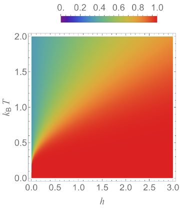
Fig . 1 d, ma : q = 3 for J = 0. No UNPC
In[]:=
Clear[q,t,h,J,Jb,mua,mub,tmin,tmax,hmin,hmax,Smax]q=3;para={J->0.,Jb->-2.,mua->1.,mub->4./3};tmin=0.001;tmax=2;hmin=0;hmax=3;Smax=1;Print["q= ",q,", para= ",para,", Log[q]= ",Log[q]]DP3ma=DensityPlotma[t,h,J,mua,Jb,mub,q]/.para,{h,hmin,hmax},{t,tmin,tmax},PlotRange{Automatic,Automatic,{0,Smax}},PlotLegendsPlaced[BarLegend[{Automatic,{0,Smax}},LabelStyle{FontSize18},LegendLayout->"Row"],{0.6,Above}],ColorFunctionScalingFalse,ColorFunction(ColorData["Rainbow"][Rescale[#,{0,Smax}]]&),PlotPoints400,MeshFunctions{#3&},Mesh{{1/q}},MeshStyle->{Dashed},MaxRecursion1,ClippingStyleAutomatic,LabelStyleDirective[Thick,FontSize18],FrameLabelStyle"",FontSize20,Style"",Italic,FontSize20(*Export["DP3ma.jpeg",DP3ma,ImageResolution300]*)
q= 3, para= {J0.,Jb-2.,mua1.,mub1.33333}, Log[q]= Log[3]
Out[]=
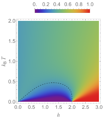
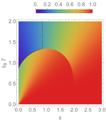
Fig . 2 Density plots of ma and mb for q = 2, 3, 10^6
Fig . 2 left panel, ma : q = 2
In[]:=
Clear[q,t,h,J,Jb,mua,mub,tmin,tmax,hmin,hmax,Smax]q=2;para={J->20.,Jb->-2.,mua->1.,mub->4./3};tmin=0.001;tmax=2;hmin=0;hmax=3;Smax=1;Print["q= ",q,", para= ",para,", Log[q]= ",Log[q]]DP2Jma=DensityPlotma[t,h,J,mua,Jb,mub,q]/.para,{h,hmin,hmax},{t,tmin,tmax},PlotRange{Automatic,Automatic,{0,Smax}},PlotLegendsPlaced[BarLegend[{Automatic,{0,Smax}},LabelStyle{FontSize18},LegendLayout->"Row"],{0.6,Above}],ColorFunctionScalingFalse,ColorFunction(ColorData["Rainbow"][Rescale[#,{0,Smax}]]&),PlotPoints400,MeshFunctions{#3&},Mesh{{1/q}},MeshStyle->{Dashed},MaxRecursion1,ClippingStyleAutomatic,LabelStyleDirective[Thick,FontSize18],FrameLabelStyle"",FontSize20,Style"",Italic,FontSize20
q= 2, para= {J20.,Jb-2.,mua1.,mub1.33333}, Log[q]= Log[2]
Out[]=
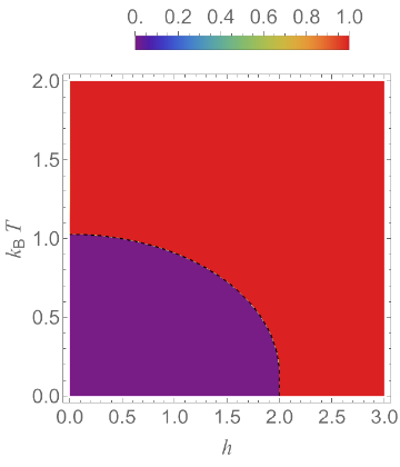
Fig . 2 right panel, mb : q = 2
In[]:=
Clear[q,t,h,J,Jb,mua,mub,tmin,tmax,hmin,hmax,Smax]q=2;para={J->20.,Jb->-2.,mua->1.,mub->4./3};tmin=0.001;tmax=2;hmin=0;hmax=3;Smax=1;Print["q= ",q,", para= ",para,", Log[q]= ",Log[q]]DP2Jmb=DensityPlotmb[t,h,J,mua,Jb,mub,q]/.para,{h,hmin,hmax},{t,tmin,tmax},PlotRange{Automatic,Automatic,{0,Smax}},PlotLegendsPlaced[BarLegend[{Automatic,{0,Smax}},LabelStyle{FontSize18},LegendLayout->"Row"],{0.6,Above}],ColorFunctionScalingFalse,ColorFunction(ColorData["Rainbow"][Rescale[#,{0,Smax}]]&),PlotPoints400,MeshFunctions{#3&},Mesh{{1/q}},MeshStyle->{Dashed},MaxRecursion1,ClippingStyleAutomatic,(*PlotLabelStyle["(a) Entropy",Large],*)LabelStyleDirective[Thick,FontSize18],FrameLabelStyle"",FontSize20,Style"",Italic,FontSize20
q= 2, para= {J20.,Jb-2.,mua1.,mub1.33333}, Log[q]= Log[2]
Out[]=
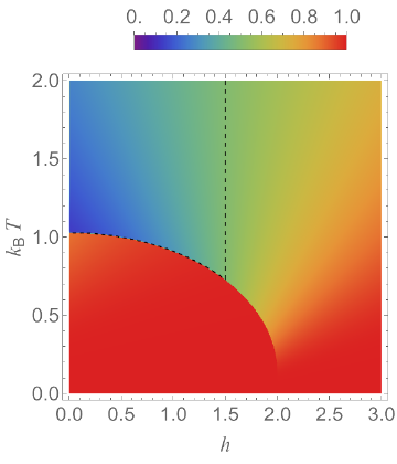
Fig . 2 left panel, ma : q = 3
In[]:=
Clear[q,t,h,J,Jb,mua,mub,tmin,tmax,hmin,hmax,Smax]q=3;para={J->20.,Jb->-2.,mua->1.,mub->4./3};tmin=0.001;tmax=2;hmin=0;hmax=3;Smax=1;Print["q= ",q,", para= ",para,", Log[q]= ",Log[q]]DP3Jma=DensityPlotma[t,h,J,mua,Jb,mub,q]/.para,{h,hmin,hmax},{t,tmin,tmax},PlotRange{Automatic,Automatic,{0,Smax}},PlotLegendsPlaced[BarLegend[{Automatic,{0,Smax}},LabelStyle{FontSize18},LegendLayout->"Row"],{0.6,Above}],ColorFunctionScalingFalse,ColorFunction(ColorData["Rainbow"][Rescale[#,{0,Smax}]]&),PlotPoints400,MeshFunctions{#3&},Mesh{{1/q}},MeshStyle->{Dashed},MaxRecursion1,ClippingStyleAutomatic,LabelStyleDirective[Thick,FontSize18],FrameLabelStyle"",FontSize20,Style"",Italic,FontSize20
q= 3, para= {J20.,Jb-2.,mua1.,mub1.33333}, Log[q]= Log[3]
Out[]=
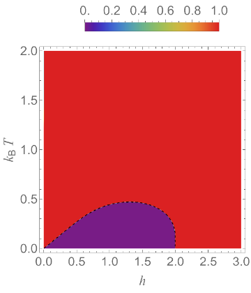
Fig . 2 right panel, mb : q = 3
In[]:=
Clear[q,t,h,J,Jb,mua,mub,tmin,tmax,hmin,hmax,Smax]q=3;para={J->20.,Jb->-2.,mua->1.,mub->4./3};tmin=0.001;tmax=2;hmin=0;hmax=3;Smax=1;Print["q= ",q,", para= ",para,", Log[q]= ",Log[q]]DP3Jmb=DensityPlotmb[t,h,J,mua,Jb,mub,q]/.para,{h,hmin,hmax},{t,tmin,tmax},PlotRange{Automatic,Automatic,{0,Smax}},PlotLegendsPlaced[BarLegend[{Automatic,{0,Smax}},LabelStyle{FontSize18},LegendLayout->"Row"],{0.6,Above}],ColorFunctionScalingFalse,ColorFunction(ColorData["Rainbow"][Rescale[#,{0,Smax}]]&),PlotPoints400,MeshFunctions{#3&},Mesh{{1/q}},MeshStyle->{Dashed},MaxRecursion1,ClippingStyleAutomatic,(*PlotLabelStyle["(a) Entropy",Large],*)LabelStyleDirective[Thick,FontSize18],FrameLabelStyle"",FontSize20,Style"",Italic,FontSize20
q= 3, para= {J20.,Jb-2.,mua1.,mub1.33333}, Log[q]= Log[3]
Out[]=
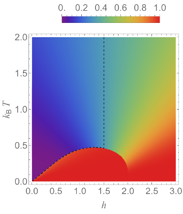
Fig . 2 left panel, ma : q = 10^6
In[]:=
Clear[q,t,h,J,Jb,mua,mub,tmin,tmax,hmin,hmax,Smax]q=10^6;para={J->20.,Jb->-2.,mua->1.,mub->4./3};tmin=0.001;tmax=2;hmin=0;hmax=3;Smax=1;Print["q= ",q,", para= ",para,", Log[q]= ",Log[q]]DP4Jma=DensityPlotma[t,h,J,mua,Jb,mub,q]/.para,{h,hmin,hmax},{t,tmin,tmax},PlotRange{Automatic,Automatic,{0,Smax}},PlotLegendsPlaced[BarLegend[{Automatic,{0,Smax}},LabelStyle{FontSize18},LegendLayout->"Row"],{0.6,Above}],ColorFunctionScalingFalse,ColorFunction(ColorData["Rainbow"][Rescale[#,{0,Smax}]]&),PlotPoints400,MeshFunctions{#3&},Mesh{{1/q}},MeshStyle->{Dashed},MaxRecursion1,ClippingStyleAutomatic,LabelStyleDirective[Thick,FontSize18],FrameLabelStyle"",FontSize20,Style"",Italic,FontSize20
q= 1000000, para= {J20.,Jb-2.,mua1.,mub1.33333}, Log[q]= Log[1000000]
Out[]=
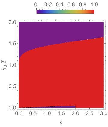
Fig . 2 right panel, mb : q = 10^6
In[]:=
Clear[q,t,h,J,Jb,mua,mub,tmin,tmax,hmin,hmax,Smax]q=10^6;para={J->20.,Jb->-2.,mua->1.,mub->4./3};tmin=0.001;tmax=2;hmin=0;hmax=3;Smax=1;Print["q= ",q,", para= ",para,", Log[q]= ",Log[q]]DP4Jmb=DensityPlotmb[t,h,J,mua,Jb,mub,q]/.para,{h,hmin,hmax},{t,tmin,tmax},PlotRange{Automatic,Automatic,{0,Smax}},PlotLegendsPlaced[BarLegend[{Automatic,{0,Smax}},LabelStyle{FontSize18},LegendLayout->"Row"],{0.6,Above}],ColorFunctionScalingFalse,ColorFunction(ColorData["Rainbow"][Rescale[#,{0,Smax}]]&),PlotPoints400,MeshFunctions{#3&},Mesh{{1/q}},MeshStyle->{Dashed},MaxRecursion1,ClippingStyleAutomatic,LabelStyleDirective[Thick,FontSize18],FrameLabelStyle"",FontSize20,Style"",Italic,FontSize20
q= 1000000, para= {J20.,Jb-2.,mua1.,mub1.33333}, Log[q]= Log[1000000]
Out[]=
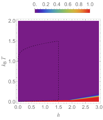
Fig . 3 : Temperature dependence of the normalized entropy S/Log[q]
In[]:=
Clear[t,h,J,mua,Jb,mub,q]para={h->1.5,J->20.,Jb->-2.,mua->1.,mub->4./3};tmin=0.001;tmax=8;ymin=-0.1;ymax=2.4;FigEntropy=Plot{entropy[t,h,J,mua,Jb,mub,2]/.para,entropy[t,h,J,mua,Jb,mub,3]/.para,entropy[t,h,J,mua,Jb,mub,100]/.para,entropy[t,h,J,mua,Jb,mub,10^6]/.para},{t,tmin,tmax},PlotRange{Automatic,{ymin,ymax}},AxesFalse,FrameTrue,PlotStyle{{color1,Dashed},{color4,Thick},{color3,Dashed},{color2,Thick},{color5,Dashed}},FrameLabelStyle"",FontSize14,Style"",FontSize14,PlotLegendsPlacedLineLegend"","","","",LabelStyle{13},LegendLayout{"Column",2},{0.65,0.2}
Out[]=
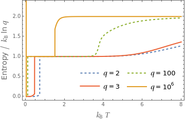
Fig . 4 left panel, ma : q = 3
In[]:=
Clear[q,t,h,J,Jb,mua,mub,tmin,tmax,hmin,hmax,Smax]q=3;para={J->20.,Jb->-2.,mua->1.,mub->2+1./3};tmin=0.001;tmax=2;hmin=0;hmax=3;Smax=1;Print["q= ",q,", para= ",para,", Log[q]= ",Log[q]]DP3Jma=DensityPlotma[t,h,J,mua,Jb,mub,q]/.para,{h,hmin,hmax},{t,tmin,tmax},PlotRange{Automatic,Automatic,{0,Smax}},PlotLegendsPlaced[BarLegend[{Automatic,{0,Smax}},LabelStyle{FontSize18},LegendLayout->"Row"],{0.6,Above}],ColorFunctionScalingFalse,ColorFunction(ColorData["Rainbow"][Rescale[#,{0,Smax}]]&),PlotPoints400,MeshFunctions{#3&},Mesh{{1/q}},MeshStyle->{Dashed},MaxRecursion1,ClippingStyleAutomatic,LabelStyleDirective[Thick,FontSize18],FrameLabelStyle"",FontSize20,Style"",Italic,FontSize20
q= 3, para= {J20.,Jb-2.,mua1.,mub2.33333}, Log[q]= Log[3]
Out[]=
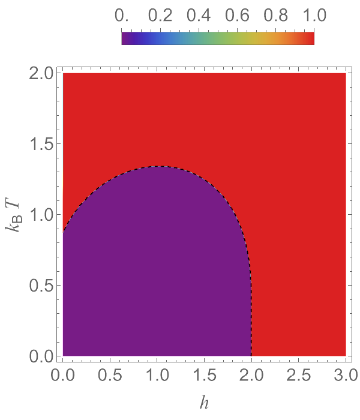
Fig . 4 right panel, mb : q = 3
In[]:=
Clear[q,t,h,J,Jb,mua,mub,tmin,tmax,hmin,hmax,Smax]q=3;para={J->20.,Jb->-2.,mua->1.,mub->2+1./3};tmin=0.001;tmax=2;hmin=0;hmax=3;Smax=1;Print["q= ",q,", para= ",para,", Log[q]= ",Log[q]]DP3Jmb=DensityPlotmb[t,h,J,mua,Jb,mub,q]/.para,{h,hmin,hmax},{t,tmin,tmax},PlotRange{Automatic,Automatic,{0,Smax}},PlotLegendsPlaced[BarLegend[{Automatic,{0,Smax}},LabelStyle{FontSize18},LegendLayout->"Row"],{0.6,Above}],ColorFunctionScalingFalse,ColorFunction(ColorData["Rainbow"][Rescale[#,{0,Smax}]]&),PlotPoints400,MeshFunctions{#3&},Mesh{{1/q}},MeshStyle->{Dashed},MaxRecursion1,ClippingStyleAutomatic,LabelStyleDirective[Thick,FontSize18],FrameLabelStyle"",FontSize20,Style"",Italic,FontSize20
q= 3, para= {J20.,Jb-2.,mua1.,mub2.33333}, Log[q]= Log[3]
Out[]=
Calculating T0 : Equations (15) - (17)
In[]:=
Clear[T0site,h,q,Jab,mua,mub,para];
Parameters
In[]:=
q=3;h=0.001;Jab=-2.;mua=1.;mub=4./3.;
Note: We work in units with k_B=1,so β=1/T
The condition for T0 is h_eff=0.
With β=1/T the effective field is
The condition for T0 is h_eff=0.
With β=1/T the effective field is
(*h_eff=h_a+T*Log[(Exp[(Jab+h_b)/T]+(q-1))/(Exp[Jab/T]+Exp[h_b/T]+(q-2))]*)
Set h_eff == 0 and solve for T.
In[]:=
T0site[h_,Jab_,mua_,mub_,q_]:=Module[{T0,T},T0=FindRoot[hmua+T*Log[(Exp[(Jab+hmub)/T]+(q-1))/(Exp[Jab/T]+Exp[hmub/T]+(q-2))]==0,{T,0.1/Log[q]}];T0[[1,2]]];T0site2[h_,Jab_,mua_,mub_,q_]:=Module[{T0,T},T0=FindRoot[hmua+T*Log[(Exp[(Jab+hmub)/T]+(q-1))/(Exp[Jab/T]+Exp[hmub/T]+(q-2))]==0,{T,1/Log[q]}];T0[[1,2]]];Print["T0 initialized from 0.1/Log[q] for h=",h,": T0 = ",T0site[h,Jab,mua,mub,q]];Print["T0 initialized from 0.1/Log[q] for h=",h,": T0 = ",T0site2[h,Jab,mua,mub,q]];T0siteh0[Jab_,muA_,muB_,q_]:=If[muB>(q-1)*muA,Jab/Log[(muB-(q-1)*muA)/(muB+muA)],0.];Print"T0 for : T0 = ",T0siteh0[Jab,mua,mub,q];
T0 initialized from 0.1/Log[q] for h=0.001: T0 = 0.000547006
T0 initialized from 0.1/Log[q] for h=0.001: T0 = 0.000547006
T0 for : T0 = 0.
In[]:=
Clear[hmin,hmax]hmin=0;hmax=2;xmin=0;xmax=3;ymin=0;ymax=2;FigT0=Plot{T0site[h,Jab,mua,mub,2],T0site[h,Jab,mua,mub,3],T0site[h,Jab,mua,mub,100]},{h,hmin,hmax},(*{t,0.144267,0.144272},*)PlotRange{{xmin,xmax},{ymin,ymax}},AxesFalse,FrameTrue,(*GridLines{{},{{0,Dashed},{1/rr-1,Dashed},{1,Dashed},{1/rr+1,Dashed}}},*)PlotStyle{{color1,Dashed},{color4,Thick},{color3,Thick},{color3,Dashed},{color4,Dotted},{color4,Dotted}},FrameLabelStyle"",Italic,FontSize14,Style"",FontSize14,PlotLegendsPlacedLineLegend"","","",LabelStyle{14},LegendLayout{"Row",3},{0.8,0.65}
Out[]=

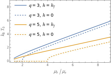
Fig . S1: 𝑇0 at (solid lines), and 𝑇0 in the limit (dashed lines) as a function of / for 𝑞 = 3 and 𝑞 = 5. 𝑇0 at is always larger, implying a 𝑇0 dome
h
f
h→0
μ
b
μ
a
h
f
In[]:=
Clear[q,h,Jab,mua,mub,mubmin,mubmax,FigT0]Jab=-2.;mua=1.;mubmin=1+1./3;mubmax=9.+1./3;xmin=1.;xmax=9;ymin=-0.2;ymax=9;FigT0=Plot{T0site[(-Jab)/mub,Jab,mua,mub,3],T0siteh0[Jab,mua,mub,3],T0site[(-Jab)/mub,Jab,mua,mub,5],T0siteh0[Jab,mua,mub,5]},{mub,mubmin,mubmax},PlotRange{{xmin,xmax},{ymin,ymax}},AxesFalse,FrameTrue,PlotStyle{{color1,Thick},{color1,Dashed},{color2,Thick},{color2,Dashed},{color4,Dotted},{color4,Dotted}},PlotPoints1000,FrameLabelStyle"",Italic,FontSize14,Style"",FontSize14,PlotLegendsPlacedLineLegend"","","","",LabelStyle{14},LegendLayout{"Row",4},{0.25,0.68}
Out[]=
New figures to address the last paragraph of End Matter
New figures to address the last paragraph of End Matter
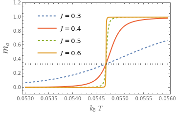
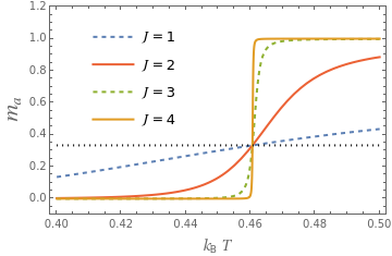
A low - UNPC results from the level crossing from to at with the crossover width . Since a type - b spin couples to one and two type - a spins in the site - and bond - decorated models, respectively, the results of the two models are similar for sufficiently large when the energy unit is set as and for the site - and bond - decorated models, respectively . It thus suffices that we focus on discussing the results for the site - decorated model in the main text . There is a subtle difference in the bond - decorated model: determined by depends on and can now slightly shift within the ultranarrow temperature window , providing a new perspective of UNPC .
T
New figure (a) : Temperature dependence of ma: is independent of for site - decoration
In[]:=
Clear[t,h,J,mua,Jb,mub,q]q=3;para={h->0.1,Jb->-2.,mua->1.,mub->4./3};tmin=0.053;tmax=0.056;ymin=-0.1;ymax=1.2;FigMaT1=Plot{ma[t,h,0.3,mua,Jb,mub,3]/.para,ma[t,h,0.4,mua,Jb,mub,3]/.para,ma[t,h,0.5,mua,Jb,mub,3]/.para,ma[t,h,0.6,mua,Jb,mub,3]/.para,1/q},{t,tmin,tmax},(*{t,0.144267,0.144272},*)PlotRange{Automatic,{ymin,ymax}},AxesFalse,FrameTrue,(*GridLines{{},{{0,Dashed},{1/rr-1,Dashed},{1,Dashed},{1/rr+1,Dashed}}},*)PlotStyle{{color1,Dashed},{color4,Thick},{color3,Dashed},{color2,Thick},{Black,Dotted}},FrameLabelStyle"",FontSize14,Style"",FontSize18,PlotLegendsPlacedLineLegend"","","","",LabelStyle{13},LegendLayout{"Column",1},{0.25,0.65}
Out[]=
New figure (b): Temperature dependence of ma: is independent of for site - decoration
In[]:=
Clear[t,h,J,mua,Jb,mub,q]q=3;para={h->1.5,Jb->-2.,mua->1.,mub->4./3};tmin=0.4;tmax=0.5;ymin=-0.1;ymax=1.2;FigMaT2=Plot{ma[t,h,1,mua,Jb,mub,3]/.para,ma[t,h,2,mua,Jb,mub,3]/.para,ma[t,h,3,mua,Jb,mub,3]/.para,ma[t,h,4,mua,Jb,mub,3]/.para,1/q},{t,tmin,tmax},(*{t,0.144267,0.144272},*)PlotRange{Automatic,{ymin,ymax}},AxesFalse,FrameTrue,(*GridLines{{},{{0,Dashed},{1/rr-1,Dashed},{1,Dashed},{1/rr+1,Dashed}}},*)PlotStyle{{color1,Dashed},{color4,Thick},{color3,Dashed},{color2,Thick},{Black,Dotted}},FrameLabelStyle"",FontSize14,Style"",FontSize18,PlotLegendsPlacedLineLegend"","","","",LabelStyle{13},LegendLayout{"Column",1},{0.25,0.65}
Out[]=
End Matter (Supplemental code)
End Matter (Supplemental code)
CITE THIS NOTEBOOK
CITE THIS NOTEBOOK
AI-co-led siscovery: half-ice, half-fire driven ultranarrow phase crossover in 1D Potts ferrimagnets
by Weiguo Yin
Wolfram Community, STAFF PICKS, July 1, 2025
https://community.wolfram.com/groups/-/m/t/3489942
by Weiguo Yin
Wolfram Community, STAFF PICKS, July 1, 2025
https://community.wolfram.com/groups/-/m/t/3489942