Universal computation or the ability to perform different tasks with the same underlying computer construction, simply by programming it differently, is a crucial part of what our world is today. In fact, the electronic device you are using to read this can mostly be considered to be a universal computer. How can we achieve the same sort of universality in the world of robotics? Is there a way that we can simulate the function of any currently existing robot with a set of identical robotic modules by simply “programming” it differently?
Parallel between universal computing and universal robotics.
As a parallel to the world of universal computation, it is hypothesized that a series of simple robotics modules could be combined to replicate the function of any other robot. In the same way that the combination of a set of simple transistors can allow a computer to perform complex calculations, an interconnected mesh of linear actuators could be capable of complicated robotic motion.
Criteria for universal robotics
To investigate the possibility of universal robotics, criteria for determining when general robotics is achieved needs to be established. In this project, it is argued that the following three characteristics are required to achieve universal robotics:
◼
Ability to control the motion of points in space
◼
Ability to resist or apply an arbitrary force at at a specific position
◼
Be capable of universal computation as a mean of controlling the robot.
It is anticipated that, in the same way that the extent of universality of a digital computer is for instance limited by the amount of memory it has, a universal robot would also have limitations based on each of the criteria listed above. One limitation would for instance be the amount of fundamental building-blocks that could be produced.
Overview
This post discusses each of the criteria for universal robotics as defined above. This includes sections on achieving arbitrary motion, resisting or applying arbitrary force and computational universality.
Arbitrary Motion
One of the goals of robotics is to move a point (or multiple points) called the end-effector, along a prescribed path. Depending on the application, it might be necessary to prescribe both the desired position and angular orientation of the end-effector. In the context of robotics, this leads to either a inverse problem: “how should the state of the respective modules change in order to move the end effector on a desired path” or the forward problem: “how does the position of the end effector change when changing the respective module states”. A module is a single fundamental building block of the overall robot. In this section the inverse problem is solved for a robot that is capable of continuous motion and the forward problem is solved for a robot with discrete states.
Inverse Kinematics
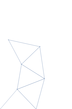
A traditional method for determining what the required module states should be for a given end effector location is inverse kinematics. This involves solving a optimisation problem. The optimal modules states are found given the desired end effector position, allowable maximum and minimum module states and collision constraints. As an example, consider a 2D robot consisting of a triangular lattice of modules connected with joints that permit rotation. A sinusoidal path is traced by the end effector without extending or contracting the modules past their limits. The states the modules can be in for this problem is a continuous range of lengths from the minimum length a linear actuator can be to the maximum length it can be. Inverse Kinematics Illustration
Out[]=
Solving the inverse problem becomes significantly harder as the number of modules (unknowns in the optimisation problem) increases.
Discrete Robotics and State Transition Diagrams
Alternatively, the end effector location can be solved as a forward problem by simulating the end effector location for a given set of module states.
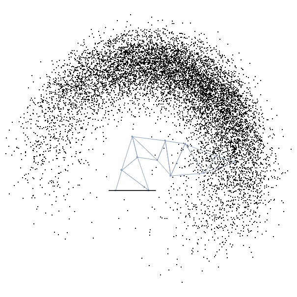
As an example, possible states for a robot consisting of a triangular lattice of modules having one of two possible states (60% ->100%) and its end-effector location is shown below. When randomly selecting the respective states of the robot’s modules to be either long or short, the end effector location can be calculated. An example of an overall robot state is plotted in blue and black dots represent the end effector positions for many randomly sampled possible robot states.
Continuous motion can be approximated by a sufficient amount of appropriately connected modules. A surrogate model can also be trained in order to try to establish a mapping between the module states and the end effector location in space.
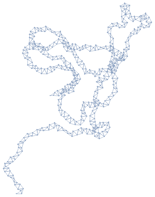
Notice that there are certain transitions between states that are not allowed. For instance, in the example robot with many modules below, the robot collides with itself. There are therefore certain constraints that determine whether the transition between two states are allowable. Other constraints could include collisions with the robots’ surroundings , exceeding the maximum force a module could resist or exert and transitions that are impossible without going to a different state first.
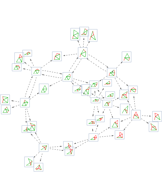
The shortest path in transitioning between two states are shown below. Notice that only a single module changes state with each time-step.
,
,
,
,
,
,
,
Rule-based Position control
An interesting opportunity for robot position control presents itself when working with modular robots that consist of modules with discrete states. Consider a 1D example of a module with discrete states where the module could either be long or short. The state of module is determined by a set a simple local rules. These rules consider the current state of a module as well as the state of its neighbours and determines the modules’ state at the next time accordingly.
The set of rules above (red=boundary,white=short, black=long) is chosen as the total length of the 1D robot changes nearly randomly as the rule updates are performed. This is done to ensure that most of the possible lengths that the robot can reach can be achieved within a relatively small amount of updates of the rule. By applying the set of rules a fixed number of times from the initial condition (modules all in short state) the robot can be extended to a known length. Since the rate at which the rule updating could occur is orders of magnitude faster than the dynamics of the robotic system, the robot would only respond after the desired number of rule updates were performed. This means that the robot could make incremental changes to its length by rapidly updating rules from an initial condition to get to the desired state. The robot can then be reset to its initial condition and the rules re-applied to transition to the next desired state.
Out[]=
Applyrule27times
Arbitrary Force
For a robot to perform a certain task its has to be able to resist the forces that are applied to it. Even in the case where a robot does not have the function of exerting a force, the force of gravity on the robot should be resisted. A few of the factors that could influence a modular robots’ ability to apply an arbitrary force include
◼
There is a maximum force that each of the modules can resist or apply
◼
The interconnected lattice of modules should be rigid
◼
As many as possible modules should contribute to resisting the applied force
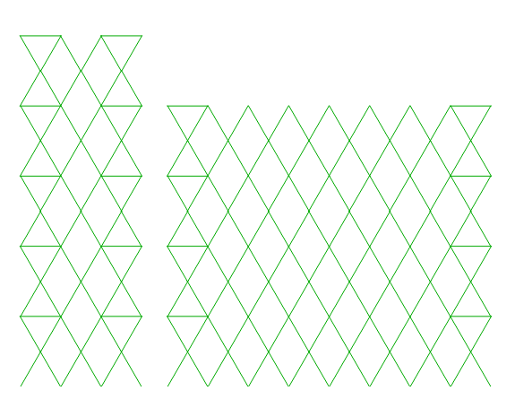
Two example lattices that could be scaled up to hypothetically apply or resist and arbitrary force is shown below. The lattice shown is rigid if the lower joint of all the lowest modules are hinged to ground. The force is applied at the end effector (top of the structure) This particular structure has no redundant members. This means that the failure of one of the components in the robot would lead to a complete failure of the robot. This lattice is chosen for this project as it is much simpler to simulate that a robot with redundant components.
By increasing the number of columns, the number of modules that act in parallel increase and as a result, the applied force (or moment it causes) that can be resisted increases (depending on where and how the force is applied). To prove this, the forces in the truss-like robot due to the applied force would have to be calculated. We could then check that the tensile or compression forces in the respective modules do not exceed their maximum allowable value. It should also be mentioned that the example shown here is not statically determinate (number of members + number of fixed degrees of freedom - 2xnumber of joints =0). A triangular lattice that distributes the force applied at the end effector through the structure and makes the structure statically determinate would have to be added to take full advantage of added columns in resisting a larger force.
And interesting result from this investigation that is not directly related to achieving arbitrary force is shown below. The examples show how the combination of fundamental building blocks could be combined to create a more complicated fundamental building block. For instance, in the image on the left, a left turn is created by stacking a series of wedge shaped layers which in turn was created by simple linear actuator modules that can either be long or short. This more complex “left turn”, “long” or “short” building block can then further be used as a building block to construct a an even more complex structure as in the image on the right.
Universal Computation
To investigate universal computation in the context of robotics, a one-dimensional problem is considered:
◼
A robot consists of serially connected modules that are capable of extending and contracting.
◼
The modules can take one of two states, long or short.
◼
Local rules determine what the state of a module would be in the next time step. For instance, if the neighbours of certain currently short module are both long, the rule might stipulate that this module should be long in the following state. All possible rules are considered in order to find the ones that would be most suitable for universal computation.
◼
At every time-step, before the local rules are applied, an additional module in the “short” state is added to the robot. One can think of the robot as systematically being assembled from one side.
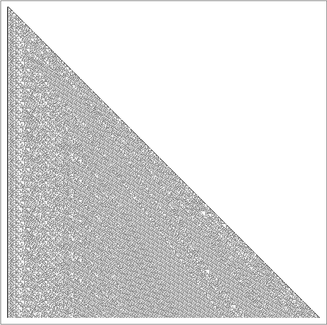
There are 2^16 = 65536 possible rules that could define the behaviour of this sort of one-dimensional robot. Looking at the evolution of theses rules, a few rules show behaviour that could indicate that this system could be capable of universal computation. For example, consider rule 51051.
Red indicate boundaries, white indicate modules in short state and black indicate modules in long state.
The evolution of the 1D robot is shown below. Notice that the number of modules that the robot is made up of grows with every update. The states of the modules (short/long) are indicated with white and grey and the boundary is shown as black . Note that the figure does not show the actual length of the 1D robot, but rather the states of the modules over time. Colliding gliders, as found in the Turing complete rule 110 elementary cellular automata (ECA110) is visible.
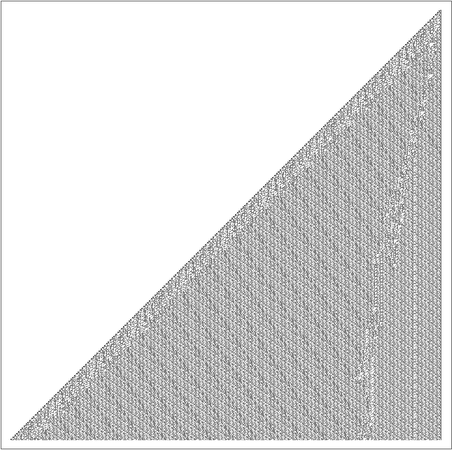
In fact, any of the elementary cellular automata could be simulated in this way. If the boundary rules are set appropriately, an all white background can be generated at every time step. As an example, we can simulate ECA 110 with rules below using the 1D robot example.
In[]:=
RulePlot[CellularAutomaton[110]]
Out[]=
We define the rules for the 1D robot to be the same as ECA 110 apart from the rules that generate the all-white background
Generalizing to 2 and 3 dimensions, it is conceivable that a modular robot with an arbitrary function could be constructed by the updating of simple rules. After a certain number of rule updates and module additions the robot would be built. In order for the robot just constructed to perform its desired function, the local rules that govern its current state could then be updated each time it has to perform a certain function.
Alternatives and Engineering Considerations
Notice that many simplification and assumptions were made in this project. The project should be viewed as a preliminary investigation into what universal robotics could mean and it is not implied that any of the simulations in this post are physically realizable.
Simulations in this investigation considered a very specific example of a robotics framework. Other alternatives include using different fundamental building blocks like rotating actuators or even actuators that change volume. Furthermore, the design of the lattice of interconnected modules will play a crucial part in the success of the modular robot. The simulations can also performed in three dimensions with the associated computational cost increase.
Some interesting engineering problems that arise when considering universal robotics include
◼
Communication with modules (Possibly electrically through lattice)
◼
Powering Components
◼
Design of connectors between modules
◼
Structural issues and vibrations
◼
Module power to size ratio tradeoffs
◼
Reliability
◼
Closed loop control
Summary
This post considered ways in which arbitrary motion and force as well as universal computation could be implemented in order to achieve general robotics.
Acknowledgement
Mentor: Philip Maymin Thank you for guidance, knowledge and shared insights during this summer school.