ABSTRACT (original article): The formation of metallic nanofilaments bridging two electrodes across an insulator is a mechanism for resistive switching. Examples of such phenomena include atomic synapses, which constitute a distinct class of memristive devices whose behavior is closely tied to the properties of the filament. Until recently, experimental investigation of the low-temperature regime and quantum transport effects has been limited. However, with growing interest in understanding the true impacts of the filament on device conductance, comprehending quantum effects has become crucial for quantum neuromorphic hardware. We discuss quantum transport resulting from filamentary switching in a narrow region where the continuous approximation of the contact is not valid, and only a few atoms are involved. In this scenario, the filament can be represented by a graph depicting the adjacency of atoms and the overlap between atomic orbitals. Using the theory of quantum graphs with locally diffusive node scattering, we calculate the scattering amplitude of charge carriers on this graph and explore the interplay between filamentary formation and quantum transport effects. CITATION (original article): Alison A. Silva, Fabiano M. Andrade, Francesco Caravelli (2024), Quantum graph models for transport in filamentary switching, arXiv:2404.06628. https://doi.org/10.48550/arXiv.2404.06628
Quantum graph models for transport in filamentary switching (QFCLaplace3)
Quantum graph models for transport in filamentary switching (QFCLaplace3)
This is the main function of our routine which connects all the other functions here defined.
The input parameters to evaluate the system are:
The input parameters to evaluate the system are:
upot: the constant potential along the edges of the quantum graph;
Dv: the dimensions of the 3D space (Dv x Dv x Dv);
singleout: a parameter that allow us to switch between:
1: single output, only one system will be evaluated and save all of the data of this single iteration such as particles positions, electric field, and so on;
0: optimized to do many iterations and save only the main data as electrical current, voltage, etc., while discards the ones that will not be used.
Here we first define our electric potential difference function, which default is defined as =0.35sin(0.5t), other parameter are defined such as the time step , number of points in the transmission probability evaluation ,...Then the initial system is defined with the function SetLeadsFlat3D, which defines both leads. With that, further calculations are made with the function PDens3DInter, where is evaluated the electric field and the filament composition by an assembly of atoms with overlapping bands. The next step is to transform this filament in a graph using GraphFromMat3, where the adjacent atoms in the system are used to define an adjacency matrix. From the adjacency matrix, we can obtain the scattering transmission in a quantum graph defined by it, for this purpose the function TQG is used. From that is possible to evaluate the current from the Landauer-Büttiker formalism, from which we got the formula for the system with two scattering channels
V
0
(dt=0.1)
(Nk=600)
I(V)dE((E)/N-(E)/M)(V)+T(E)
G
0
∞
∫
-∞
f
L
f
R
h
2
2
e
σ
0
where is the conductance quantum, (E) and (E) are obtained from the Fermi-Dirac distribution, which can be evaluated with the chempot function, is an additional conductivity of the device, which can be either constant or voltage-dependent, and is the transmission probability obtained from the quantum graph scattering transmission evaluation. From these evaluations, the function returns Vt: a list containing the voltage for each step of time, It and Ifp: the current as function of time for a trivial or a Frenkel-Poole insulator, respectively, and Ampt: a list with the scattering transmission probability of the quantum graph modeled by the filament for each step of time.
G
0
f
L
f
R
σ
0
T(E)
Initial boundaries (SetLeadsFlat3D)
Initial boundaries (SetLeadsFlat3D)
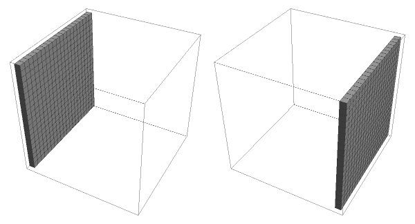
In this function the objective is to define the initial boundaries of the system without filaments. Here we first define the dimensions of the system with the parameters H, W and Dv, and then we define the top and bottom planes of the cube as two plates which are obtained by the following function:
In[]:=
SetLeadsFlat3D[H_,W_,Dv_]:=Module[{NpTop=ConstantArray[0,{W,Dv,H}],NpBottom=ConstantArray[0,{W,Dv,H}]},NpTop〚All,All,1〛=ConstantArray[1,{H,W}];NpBottom〚All,All,-1〛=ConstantArray[1,{H,W}];{NpTop,NpBottom}];
It will return a list of two 3D arrays, one for each plane, which will define the leads of our system.
Example:
Example:
Lets define a system with dimensions 20 x 20 x 20, thus we have
In[]:=
exSetLeadsFlat3D=SetLeadsFlat3D[20,20,20];
Now can we visualize them with
In[]:=
GraphicsRow[ArrayPlot3D/@exSetLeadsFlat3D]
Out[]=
Electric Field evaluation (LaplaceSolver3D)
Electric Field evaluation (LaplaceSolver3D)
In this function we aim to obtain the electric field between the two planes that define the leads in our system. To obtain that we need the following parameters:
V0: the electric difference potential between the leads;
MyBoundaryTop and MyBoundaryBottom: the two leads with +V0/2 and -V0/2 electric potentials respectively;
First we define a 3D array containing the initial potential in all of the discrete points of the system, being in the top plane, in the bottom one and elsewhere. Then for all points, except the ones in the border of the defined space, we evaluate its electric potential by taking the mean value of six neighbor points, two for each direction (one before and one after). This iteration will be realized until the difference between the new and the last iteration is less or equal than the defined error parameter.Finally the electric field is evaluated from the potential matrix, by taking the differences between the electric potential values in each directions, as an discrete gradient. The function constructed for this purpose is the one as follows:
+/2
V
0
-/2
V
0
0
In[]:=
LaplaceSolver3D[V0_,MyBoundaryTop_,MyBoundaryBottom_]:=Module{xdim,ydim,zdim,VNow,VPrev,error,ex,ey,ez},xdim=Dimensions[MyBoundaryTop]1-1;ydim=Dimensions[MyBoundaryTop]2-1;zdim=Dimensions[MyBoundaryTop]3-1;VPrev=ConstantArray[0,{xdim+1,ydim+1,zdim+1}];VNow=V0(MyBoundaryTop-MyBoundaryBottom);error=Max[Abs[VNow-VPrev]];VPrev=VNow;Whileerror>0.01`,DoIfMyBoundaryTopi,j,k0&&MyBoundaryBottomi,j,k0,VNowi,j,k=(VPrev〚i-1,j,k〛+VPrev〚i+1,j,k〛+VPrev〚i,j-1,k〛+VPrev〚i,j+1,k〛+VPrev〚i,j,k-1〛+VPrev〚i,j,k+1〛);;,{i,2,xdim},{j,2,ydim},{k,2,zdim};error=Max[Abs[VNow-VPrev]];VPrev=VNow;;MatrixPosaux=VNow;ez=MapAt[0.5`#1&,ArrayPad[Differences[VNow,{0,0,1}],{{0,0},{0,0},{0,1}}]+ArrayPad[Differences[VNow,{0,0,1}],{{0,0},{0,0},{1,0}}],{All,All,2;;-2}];ey=MapAt[0.5`#1&,ArrayPad[Differences[VNow,{0,1,0}],{{0,0},{0,1},{0,0}}]+ArrayPad[Differences[VNow,{0,1,0}],{{0,0},{1,0},{0,0}}],{All,2;;-2,All}];ex=MapAt[0.5`#1&,ArrayPad[Differences[VNow,{1,0,0}],{{0,1},{0,0},{0,0}}]+ArrayPad[Differences[VNow,{1,0,0}],{{1,0},{0,0},{0,0}}],{2;;-2,All,All}];{ex,ey,ez};
1
2
1
6
The electric field is returned in the form {ex, ey, ez} being a list of three 3D arrays, each of these arrays the component for the electric field in the directions x, y and z for each discrete point of the defined system.
Example:
Example:
Lets define a x x system by using the function SetLeadsFlat3D, which will give us the two leads.
20
20
20
In[]:=
exSetLeadsFlat3D=SetLeadsFlat3D[20,20,20];
Also we will plot both leads as top and bottom planes, with potential and , respectively.
+0.5
-0.5
In[]:=
ArrayPlot3D[Transpose[.5exSetLeadsFlat3D[[1]]-.5exSetLeadsFlat3D[[2]],1<->3],PlotLegends->Automatic]
Out[]=

Now let us evaluate the electric field between these leads with the LaplaceSolver3D, by defining V0=1:
In[]:=
exLaplaceSolver3D=LaplaceSolver3D[1,exSetLeadsFlat3D[[1]],exSetLeadsFlat3D[[2]]];
It is interesting to rearrange the outputs in a single array,
In[]:=
exElectricField=Table[{-exLaplaceSolver3D[[1]]〚i,j,k〛,-exLaplaceSolver3D[[2]]〚i,j,k〛,-exLaplaceSolver3D[[3]]〚i,j,k〛},{i,20},{j,20},{k,20}];
this allow us to plot the electric field with the following command :
In[]:=
ListVectorPlot3D[exElectricField,VectorScaling->Automatic,VectorMarkers->"Arrow",VectorSizes->{0,.25},VectorPoints->All,PlotRange->All]
Out[]=

Particles interaction and filaments construction (PDens3DInter)
Particles interaction and filaments construction (PDens3DInter)
This function aims to model the filaments construction, for that we must define the initial parameters:
treetopl and treebottoml: list of coordinates {x,y,z} for each component of the filament, which will become a vertex of the graph; Initially both are defined as an empty list and will grow as this function is re utilized in a loop; The difference between top and bottom are due the particle will start from different leads according to the electric potential in each lead;
MatrixPos: An array with the dimension of all the possible positions. As a particle become part of the filament, an label will be give to it and stored in this array in the same position as the particle;
nnodes: number of vertices in the graph that model the filament;
T: a time step parameter;
H and W: parameters related with the dimension of the system, W x W x H (along with this routine all of three are the same);
pdecay: parameter related to the probability of an vertex be removed of the graph or the decay of some part of the filament;
V: the electric potential difference at that step of time;
Ppos: Position of all the particles that are not connected to the filament (free particles between the leads), this list contains for each particle, its early position and its actual position;
TreeTop0, TreeBottom0, TreeTop and TreeBottom: the early and new matrices which storage which discrete positions are already occupied and are used to verify if the free particles are close enough to be attached to the filament.
In this program, from the initial parameters, a random number of particles, also controlled by a density parameter and by the size of the system, is generated from one lead. These particles also receive random directions of propagation. These particles will interact with the electric field calculated with the function LaplaceSolver3D. When some particle is detected to be close enough to the other lead or to some other particle in the filament, it will also become part of the filament in that position. A label will be given to this particle and it will be registered to after transform this filament into a graph. Finally the PDens3DInter returns some arrays that describe the configuration of the system at that step of time, which can be used in a loop to the next iterations.
Graph construction from filament position(GraphFromMat3)
Graph construction from filament position(GraphFromMat3)
This function uses the input MatrixPos which non zeros elements corresponds to particles that is part of the filament, being the position of in the array related to it real position in the system. First we define each lead as the vertices and 2, and then the number of particles in the filament is evaluated as the non zero elements in MatrixPos, assigning to each of them a label.Then a matrix - being the number of particles in the filament plus the two leads - with all elements zeros is constructed, this will become the adjacency matrix. A scan is done on the entire array and for each adjacent non zero element in the array, this adjacency matrix has the following replacement in its elements: ==1, being and the label of these particles. Also the position where each vertex was is stored to further be possible to draw the graph.Finally this function returns parameters related to the number of vertices connected to each leads, the adjacency matrix and the spatial position of each vertex.
1
(n×n)
A
i,j
A
j,i
In[]:=
GraphFromMat3[MatrixPos_]:=Module{kv,rv,m,MatrixPosNew=MatrixPos,H=Dimensions[MatrixPos]〚3〛,W=Dimensions[MatrixPos]〚1〛,bl={},tl={},A,x,y,z,posidxs,nverts},MatrixPosaux2=MatrixPosNew;posidxs=Cases[Flatten[MatrixPosNew〚All,All,2;;-2〛],Except[0]];nverts=Length[posidxs];A=ConstantArray[0,{nverts+2,nverts+2}];x=ConstantArray[0,nverts+2];y=ConstantArray[0,nverts+2];z=ConstantArray[0,nverts+2];x1=;y1=;z1=1;x2=;y2=;z2=H;If[nverts>0,Do[If[MatrixPosNew〚iaux,jaux,kaux〛>0,kv=Position[posidxs,MatrixPosNew〚iaux,jaux,kaux〛]〚1,1〛+2;If[kaux2,AppendTo[tl,kv];A〚1,kv〛=A〚kv,1〛=1;];If[kauxH-1,AppendTo[bl,kv];A〚2,kv〛=A〚kv,2〛=1;];x〚kv〛=iaux;y〚kv〛=jaux;z〚kv〛=kaux;(If[MatrixPosNew〚#1,#2,kaux〛>0,rv=Position[posidxs,MatrixPosNew〚#1,#2,kaux〛]〚1,1〛+2;A〚rv,kv〛=A〚kv,rv〛=1;]&)@@@Tuples[{{iaux-1,iaux+1},{jaux-1,jaux+1}}];If[2<kaux<W-1,Do[(If[MatrixPosNew〚#1,#2,kaux+kaux2〛>0,rv=Position[posidxs,MatrixPosNew〚#1,#2,kaux+kaux2〛]〚1,1〛+2;A〚rv,kv〛=A〚kv,rv〛=1;]&)@@@Tuples[{{iaux-1,iaux,iaux+1},{jaux-1,jaux,jaux+1}}],{kaux2,-1,1,2}];];];,{iaux,2,W-1},{jaux,2,W-1},{kaux,2,H-1}];,A={{0,0},{0,0}};bl={};tl={};];{bl,tl,A,x,y,z};
W
2
W
2
W
2
W
2
Transmission in a Quantum Graph (TQG)
Transmission in a Quantum Graph (TQG)
Here we explain the method for calculate the transmission in a quantum graph. First we should define the parameters that will be utilized to evaluate this function.
adjM: This first parameter is the Adjacency matrix from a graph that defines the connectivity of the target quantum graph;
ve and vs: As the scattering transmission in a quantum system is obtained from one scattering channel to another, we define two parameters, and , which are vertices where the entrance and exit scattering channels are attached to respectively;
z: This last parameter is related to the metrics defined along the edges, as in this work we consider all edges with the same length, we can define it an variable , where is the wavenumber of the particle and is the length of the edges, and obtain an expression for the scattering transmission as function of , or alternatively, obtain numerical results by assigning numerical values to this parameter;
From these parameter is possible to obtain the transmission in a quantum graph by the following steps. First we obtain a list which contain the degrees of the vertices in the graph. It is obtained by taking the sum of each row in its adjacency matrix
d
j
N
∑
j=1
A
i,j
where is the size of this adjacency matrix. As the scattering channels increase the vertex degree, we do an increment in the positions defined by and .With the degrees defined we are able to obtain the scattering amplitudes in each vertex, as we utilize the Neumann-Kirchhoff boundary condition in all of them, they are defined by
t
j
2
d
j
r
j
2
d
j
with , and for , and . Now we can generate an equation system of families of paths along the edges of the quantum graph that is defined by
p
ij
∑
l=
n
N
j
z
ij
[{j,l},{i,j}]
σ
j
A
jl
p
jl
δ
jn
z
in
[,{i,n}]
e
σ
n
Through this method, the Green function of this system is obtained as
Where is the transmission amplitude of this quantum graph which is obtained by solving the equation system for families of paths in the quantum graph
Thus, with these steps described, the following function was constructed, which returns the transmission amplitude of the quantum graph
In[]:=
TQG[adjM_,ve_,vs_,z_]:=Module{inc,d,t,r,ps,eqs,lAdjm,p,eq,sol,T1},Clear[p,eq,ps,eqs];d=Total[adjM,{1}];dve+=1;dvs+=1;t=If#1>1,,0&/@d;r=If#1>1,-1,If[#11,1,0]&/@d;ps={};eqs={};lAdjm=Length[adjM];DoDoIfn≠m,IfadjMm,n≠0,ps=Join[ps,{p[m,n]}];eqs=Joineqs,p[m,n]-zrnp[n,m]+tnIf[jjm||adjM〚n,jj〛0,0,p[n,jj]]+0;;;,{n,1,lAdjm};,{m,1,lAdjm};sol=Chop[Solve[eqs,ps]];T1=ChopSimplifytveadjMve,jjp[ve,jj]+/.sol1;T1;
2
#1
2
#1
lAdjm
∑
jj=1
δ
vs,n
lAdjm
∑
jj=1
δ
vs,ve
Example:
Example:
First let us define a graph like the Wheel graph with 5 vertices:
In[]:=
exG=WheelGraph[5,VertexLabels->Automatic]
Out[]=
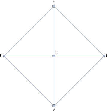
Now we take its adjacency matrix and print it:
In[]:=
exAdjM=AdjacencyMatrix[exG];exAdjM//MatrixForm
Out[]//MatrixForm=
0 | 1 | 1 | 1 | 1 |
1 | 0 | 1 | 0 | 1 |
1 | 1 | 0 | 1 | 0 |
1 | 0 | 1 | 0 | 1 |
1 | 1 | 0 | 1 | 0 |
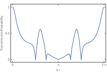
Finally we evaluate its Transmission amplitude, taking and ,
In[]:=
exTQG=TQGexAdjM,1,2,
kl
Out[]=
-
6(3+7+10+10+7+3)
kl
kl
2kl
3kl
4kl
5kl
-90-90-139-27-14+66+27+27
kl
2kl
3kl
4kl
5kl
6kl
7kl
And now we can plot the transmission probability as function of
In[]:=
Plot[Abs[exTQG/.{kl->x}],{x,0,2π},Frame->True,FrameStyle->Thick,FrameTicks->{{{0,.5,1},{{0,""},{.5,""},{1,""}}},{{0,Pi,2Pi},{{0,""},{Pi,""},{2Pi,""}}}},FrameLabel->{"k l","Transmission Probability"}]
Out[]=
Other quantities and functions (qe, me, ℏ, chempot, DecayM2)
Other quantities and functions (qe, me, ℏ, chempot, DecayM2)
In this section we define some quantities used along the programs and some small functions.qe, me and ℏ: electron charge, electron mass and the reduced Planck constant.DecayM2: function used to random remove some particles of the filament, by randomly replacing some elements of the matrix of positions for the filaments to .chempot: returns the Fermi-Dirac distribution for given particles energy en, chemical potential μ, and T the given temperature times the Boltzmann constant.
In[]:=
qe=QuantityMagnitude["Electron Charge","SIBase"]//N;me=QuantityMagnitude["Electron Mass","SIBase"];ℏ=QuantityMagnitude["Reduced Planck Constant","SIBase"]//N;DecayM2[M_,MatrixPos_,p_,nnodes_]:=Module[{Md=M,MatrixPosNew=MatrixPos,nnodesnew=nnodes},Do[If[Md〚i,j,k〛≠0&&RandomReal[]<p,Md〚i,j,k〛=0;MatrixPosNew〚i,j,k〛=0;nnodesnew=nnodesnew-1;];,{i,1,Dimensions[Md]〚1〛},{j,1,Dimensions[Md]〚2〛},{k,1,Dimensions[Md]〚3〛}];{Md,MatrixPosNew,nnodesnew}];chempot[en_,μ_,T_]:=;
1
Exp+1
en-μ
T
Examples and data plots
Examples and data plots
Single iteration with video generation
Single iteration with video generation
First we define the list with the data that we will use and run the function QFCLaplace3 with the target parameters, e.g. here will be defined as potential in the edges upot=0, Dv=20 and singleout=1 to save all the data for a single iteration, which includes electric potential vectors, particles positions,... All the data is automatic stored in the same file as this notebook.
In[]:=
Vtaux={};Itaux={};Ifpaux={};Pposaux={};vecs={};graphaux={};AmpListaux={};QFCLaplace3[0.00,20,1];
After running this, now we can generate the videos from these data. Following we will describe each of the plots and the code to generate them.
Note: “MaTeX” package is needed.
Note: “MaTeX” package is needed.
In[]:=
Needs["MaTeX`"];SetOptions[MaTeX,"Preamble"->{"\\usepackage{helvet}","\\renewcommand{\\familydefault}{\\sfdefault}"},FontSize->12];SetDirectory[NotebookDirectory[]];
Voltage versus time
vt=Transpose[{.1Range[629],ReadList["Dim=20_u=0._V_t.csv"][[1]]}];x1ticks=With[{ticks=Range[0,60,15]},{#,None}&/@ticks];x2ticks=With[{ticks=Range[0,60,15]},{#,None}&/@ticks];y1ticks=With[{ticks=Range[-.4,.4,.4]},{#,MaTeX[ToString[TeXForm[NumberForm[#,{2,1}]]],"DisplayStyle"->False,Magnification->2]}&/@ticks];y2ticks=With[{ticks=Range[-.4,.4,.4]},{#,None}&/@ticks];
In[]:=
videoVt=AnimationVideo[ListLinePlot[Take[vt,i],PlotRange->{{-1,64},{-0.45,0.45}},Frame->True,FrameTicks->{{y1ticks,y2ticks},{x1ticks,x2ticks}},FrameLabel->{None,MaTeX["\\text{Voltage, } V(V)",Magnification->2]},AspectRatio->1,FrameStyle->Directive[Darker[Blue,1],Thick],ImageSize->72(235)/12,ColorFunction->Function[{x,y},ColorData["BrightBands"][Floor[(x)/(4π)]/Ceiling[62.9/(4π)]]],ColorFunctionScaling->False],{i,1,629,1},FrameRate->10]
Out[]=
In[]:=
Export["VideoVt.mp4",videoVt]
Out[]=
VideoVt.mp4
Current versus time
In[]:=
it=Transpose[{.1Range[629],ReadList["Dim=20_u=0._I_t.csv"][[1]]}];x1ticks=With[{ticks=Range[0,60,15]},{#,MaTeX[ToString[TeXForm[NumberForm[#,{2,0}]]],"DisplayStyle"->False,Magnification->2]}&/@ticks];x2ticks=With[{ticks=Range[0,60,15]},{#,None}&/@ticks];y1ticks=Withticks=Range[-4.5*,4.5*,4.5*],#,MaTeXToString[TeXForm[NumberForm[N[#],{2,1}]]],"DisplayStyle"->False,Magnification->2&/@ticks;y2ticks=Withticks=Range[-4.5*,4.5*,4.5*],{#,None}&/@ticks;
-6
10
-6
10
-6
10
6
10
-6
10
-6
10
-6
10
In[]:=
videoIt=AnimationVideoListLinePlotTake[it,i],PlotRange->{{-1,64},{-5,5}},Frame->True,FrameTicks->{{y1ticks,y2ticks},{x1ticks,x2ticks}},FrameLabel->{MaTeX["\\text{Time, } t(s)",Magnification->2],MaTeX["\\text{Current, } I(\\mu A)",Magnification->2]},AspectRatio->1,FrameStyle->Directive[Darker[Blue,1],Thick],ImageSize->72(235)12,ColorFunction->Function[{x,y},ColorData["BrightBands"][Floor[(x)/(4π)]/Ceiling[62.9/(4π)]]],ColorFunctionScaling->False,{i,1,629,1},FrameRate->10
-6
10
-6
10
Out[]=
In[]:=
Export["VideoIt.mp4",videoIt];
Current (Frenkel-Poole insulator) versus time
In[]:=
ift=Transpose[{.1Range[629],ReadList["Dim=20_u=0._If_t.csv"][[1]]}];x1ticks=x1ticks=With[{ticks=Range[0,60,15]},{#,MaTeX[ToString[TeXForm[NumberForm[#,{2,0}]]],"DisplayStyle"->False,Magnification->2]}&/@ticks];x2ticks=With[{ticks=Range[0,60,15]},{#,None}&/@ticks];y1ticks=Withticks=Range[-10.5*,10.5*,10.5*],#,MaTeXToString[TeXForm[NumberForm[#,{2,1}]]],"DisplayStyle"->False,Magnification->2&/@ticks;y2ticks=Withticks=Range[-10.5*,10.5*,10.5*],{#,None}&/@ticks;
-6
10
-6
10
-6
10
6
10
-6
10
-6
10
-6
10
In[]:=
videoIft=AnimationVideoListLinePlotTake[ift,i],PlotRange->{{-1,64},{-11,11}},Frame->True,FrameTicks->{{y1ticks,y2ticks},{x1ticks,x2ticks}},FrameLabel->{MaTeX["\\text{Time, } t(s)",Magnification->2],MaTeX["\\text{Current, } I(\\mu A)",Magnification->2]},AspectRatio->1,FrameStyle->Directive[Darker[Blue,1],Thick],ImageSize->72(235)12,ColorFunction->Function[{x,y},ColorData["BrightBands"][Floor[(x)/(4π)]/Ceiling[62.9/(4π)]]],ColorFunctionScaling->False,{i,1,629,1},FrameRate->10
-6
10
-6
10
Out[]=
In[]:=
Export["VideoIft.mp4",videoIt];
Current versus voltage
In[]:=
ivt=Transpose[{ReadList["Dim=20_u=0._V_t.csv"][[1]],ReadList["Dim=20_u=0._I_t.csv"][[1]]}];x1ticks=With[{ticks=Range[-.4,.4,.4]},{#,MaTeX[ToString[TeXForm[NumberForm[#,{2,1}]]],"DisplayStyle"->False,Magnification->2]}&/@ticks];x2ticks=With[{ticks=Range[-.4,.4,.4]},{#,None}&/@ticks];y1ticks=Withticks=Range[-4.5*,4.5*,4.5*],#,MaTeXToString[TeXForm[NumberForm[N[#],{2,1}]]],"DisplayStyle"->False,Magnification->2&/@ticks;y2ticks=Withticks=Range[-4.5*,4.5*,4.5*],{#,None}&/@ticks;
-6
10
-6
10
-6
10
6
10
-6
10
-6
10
-6
10
In[]:=
videoIvt=AnimationVideoListLinePlotPartition[Take[ivt,i],UpTo[126]],PlotRange->{{-0.47,0.47},{-5*,5*}},Frame->True,FrameTicks->{{y1ticks,y2ticks},{x1ticks,x2ticks}},FrameLabel->{MaTeX["V(V)",Magnification->2],MaTeX["I(\\mu A)",Magnification->2]},AspectRatio->1,FrameStyle->Directive[Darker[Blue,1],Thick],Epilog->{Black,PointSize[Medium],Point[ivt[[i]]]},ImageSize->72(235)12,PlotStyle->Table[ColorData["BrightBands"][Floor[((4π-.1)j)/(4π)]/Ceiling[62.9/(4π)]],{j,1,10}],{i,1,629,1},FrameRate->10
-6
10
-6
10
Out[]=
In[]:=
Export["VideoIVt.mp4",videoIvt];
Current (Frenkel-Poole) versus time
In[]:=
ifvt=Transpose[{ReadList["Dim=20_u=0._V_t.csv"][[1]],ReadList["Dim=20_u=0._If_t.csv"][[1]]}];x1ticks=With[{ticks=Range[-.4,.4,.4]},{#,MaTeX[ToString[TeXForm[NumberForm[#,{2,1}]]],"DisplayStyle"->False,Magnification->2]}&/@ticks];x2ticks=With[{ticks=Range[-.4,.4,.4]},{#,None}&/@ticks];y1ticks=Withticks=Range[-10.5*,10.5*,10.5*],#,MaTeXToString[TeXForm[NumberForm[N[#],{2,1}]]],"DisplayStyle"->False,Magnification->2&/@ticks;y2ticks=Withticks=Range[-10.5*,10.5*,10.5*],{#,None}&/@ticks;
-6
10
-6
10
-6
10
6
10
-6
10
-6
10
-6
10
In[]:=
videoIfvt=AnimationVideoListLinePlotPartition[Take[ifvt,i],UpTo[126]],PlotRange->{{-0.47,0.47},{-11,11}},Frame->True,FrameTicks->{{y1ticks,y2ticks},{x1ticks,x2ticks}},FrameLabel->{MaTeX["V(V)",Magnification->2],MaTeX["I(\\mu A)",Magnification->2]},AspectRatio->1,FrameStyle->Directive[Darker[Blue,1],Thick],Epilog->{Black,PointSize[Medium],Point[ifvt[[i]]]},ImageSize->72(235)12,PlotStyle->Table[ColorData["BrightBands"][Floor[((4π-.1)j)/(4π)]/Ceiling[62.9/(4π)]],{j,1,10}],{i,1,629,1},FrameRate->10
-6
10
-6
10
Out[]=
In[]:=
Export["VideoIfVt.mp4",videoIfvt]
Out[]=
VideoIfVt.mp4
Transmission
In[]:=
tent=ReadList["Dim=20_u=0._T_en_t.csv"];tentchem=ReadList["Dim=20_u=0._T_en_t_Chem.csv"];
In[]:=
x1ticks={{0.0,MaTeX[ToString[TeXForm[NumberForm[0.,{2,2}]]],"DisplayStyle"->False,Magnification->2]},{0.175/2,MaTeX[ToString[TeXForm[NumberForm[0.25,{2,2}]]],"DisplayStyle"->False,Magnification->2]},{0.175,MaTeX[ToString[TeXForm[NumberForm[0.5,{2,2}]]],"DisplayStyle"->False,Magnification->2]}};x2ticks=With[{ticks=Range[0.,0.175,.175/2]},{#,None}&/@ticks];y1ticks=With[{ticks=Range[0.,1.,0.5]},{#,MaTeX[ToString[TeXForm[NumberForm[#,{2,1}]]],"DisplayStyle"->False,Magnification->2]}&/@ticks];y2ticks=With[{ticks=Range[0.,1.,0.5]},{#,None}&/@ticks];
In[]:=
videoTkt=AnimationVideo[ListLinePlot[{Take[tent[[i]],-300]},PlotRange->{{-.005,0.18},{-.05,1.05}},Frame->True,FrameTicks->{{y1ticks,y2ticks},{x1ticks,x2ticks}},FrameLabel->{{MaTeX["T",Magnification->2],""},{MaTeX["E/V_0",Magnification->2],""}},AspectRatio->1,FrameStyle->Directive[Darker[Blue,1],Thick],ImageSize->72(235)/12],{i,1,629,1},FrameRate->10]
Out[]=
In[]:=
Export["VideoTkt.mp4",videoTkt];
Filament formation
In[]:=
vecs=ReadList["Dim=20_u=0.vecs.csv"];
In[]:=
Pposaux=ReadList["Dim=20_u=0.Ppos.csv"];
In[]:=
Adj=ReadList["Dim=20_u=0.Adj.csv"];
video3D=AnimationVideo[Show[{ListVectorPlot3D[vecs[[i]],VectorScaling->Automatic,VectorMarkers->"Arrow",VectorSizes->{0,.25},VectorPoints->All,PlotRange->All,ImageSize->600],If[Length[Pposaux[[i]]]>0,Graph[Range[Length[Pposaux[[i]]]],{},VertexCoordinates->Transpose[{Pposaux[[i]][[All,1,1]],Pposaux[[i]][[All,2,1]],Pposaux[[i]][[All,3,1]]}],VertexSize->{{.5,.5}},VertexStyle->{Opacity[.75],Gray}],Graph[Range[1],{},VertexCoordinates->{{-10,-10,-10}},VertexSize->{{.5,.5}},VertexStyle->{Opacity[.75],Gray}]],If[Length[Pposaux[[i]]]>0,Graph[Range[Length[Pposaux[[i]]]],{},VertexCoordinates->Transpose[{Pposaux[[i]][[All,1,2]],Pposaux[[i]][[All,2,2]],Pposaux[[i]][[All,3,2]]}],VertexSize->{{.5,.5}},VertexStyle->{Opacity[.75],LightGray}],Graph[Range[1],{},VertexCoordinates->{{-10,-10,-10}},VertexSize->{{.5,.5}},VertexStyle->{Opacity[.75],LightGray}]],AdjacencyGraph[Adj[[i,1]],VertexSize->{{.5,.5}},VertexStyle->{Opacity[.75],1->{Blue},2->{Red}},VertexCoordinates->Adj[[i,2]],ImageSize->100]},Ticks->None],{i,1,629,1},FrameRate->10];
Out[]=
In[]:=
Export["video3D.mp4",video3D];
Plots combine
In[]:=
v1=Import["VideoVt.mp4"];v2=Import["VideoIt.mp4"];v3=Import["VideoIVt.mp4"];v4=Import["VideoTkt.mp4"];v5=Import["video3D.mp4"];
In[]:=
grid=GridVideo[{{GridVideo[{{v1},{v2}},PaddingSize->100,Background->None],v5},{Missing[],GridVideo[{{v3,v4}},PaddingSize->100,Spacings->10,Background->None]}},Background->None]
Out[]=
In[]:=
Export["video_sigma_const_layout1.mp4",grid]
Out[]=
video_sigma_const_layout1.mp4
In[]:=
grid=GridVideo[{{GridVideo[{{v1},{v2}},PaddingSize->100,Background->None],v5,GridVideo[{{v3},{v4}},PaddingSize->100,Spacings->10,Background->None]}},Background->None];
Out[]=
In[]:=
Export["video_sigma_const_layout2.mp4",grid]
Out[]=
video_sigma_const_layout2.mp4
In[]:=
v1=Import["VideoVt.mp4"];v2=Import["VideoIft.mp4"];v3=Import["VideoIfVt.mp4"];v4=Import["VideoTkt.mp4"];v5=Import["video3D.mp4"];
In[]:=
grid=GridVideo[{{GridVideo[{{v1},{v2}},PaddingSize->100,Background->None],v5},{Missing[],GridVideo[{{v3,v4}},PaddingSize->100,Spacings->10,Background->None]}},Background->None]
Out[]=
In[]:=
Export["video_sigma_exp_layout1.mp4",grid]
Out[]=
video_sigma_exp_layout1.mp4
In[]:=
grid=GridVideo[{{GridVideo[{{v1},{v2}},PaddingSize->100,Background->None],v5,GridVideo[{{v3},{v4}},PaddingSize->100,Spacings->10,Background->None]}},Background->None];
Out[]=
In[]:=
Export["video_sigma_exp_layout2.mp4",grid]
Out[]=
video_sigma_exp_layout2.mp4
CITE THIS NOTEBOOK
CITE THIS NOTEBOOK
Quantum graph models for transport in filamentary switching
by Alison A. Silva, Fabiano M. Andrade & Francesco Caravelli
Wolfram Community, STAFF PICKS, December 3, 2024
https://community.wolfram.com/groups/-/m/t/3332704
by Alison A. Silva, Fabiano M. Andrade & Francesco Caravelli
Wolfram Community, STAFF PICKS, December 3, 2024
https://community.wolfram.com/groups/-/m/t/3332704