ABSTRACT (original article): Hotspots, often characterized as pointlike emissions, frequently appear near black holes with significantly enhanced luminosity compared to the surrounding accretion flow. Notably, such hotspots are regularly observed near the black hole at the center of the Milky Way. Light rays emitted from these sources follow complex trajectories around the black hole before reaching distinct locations on the observer’s image plane. Precisely resolving both direct emissions and their higher-order images—despite the latter’s intensity suppression—is essential for extracting detailed spacetime information, including the black hole’s mass, spin, and inclination angle. To improve the accuracy and efficiency of hotspot modeling, we develop a forward ray tracing method based on the analytic integral solution of Kerr geodesics, leveraging conserved quantities. Our approach traces geodesics from a given emission point near the black hole to a distant observer, effectively capturing multiple images with a tailored parametrization scheme for root-finding. By perturbing these geodesics, we map finite-size emissions to distinct regions on the image plane, enabling the quantification of image shapes and amplification rates. This method not only enhances the identification of strongly lensed photons from black holes but also enables efficient spacetime tomography and hotspot localization, leveraging observations from the Event Horizon Telescope and its upcoming next-generation upgrades. CITATION (original article): Lihang Zhou, Zhen Zhong, Yifan Chen, Vitor Cardoso (2025), Forward ray tracing and hot spots in Kerr spacetime, Phys. Rev. D 111, 064075. https://doi.org/10.1103/PhysRevD.111.064075
Github: https://github.com/AuroraDysis/KerrP2P
Github: https://github.com/AuroraDysis/KerrP2P
KerrP2P is a software designed for forward ray tracing in Kerr spacetime. It is specifically tailored to efficiently calculate multiple null geodesics between designated “source” and “observer” points, locate apparent positions of the corresponding images, and quantify their shapes. Detailed information can be found in the paper Forward Ray Tracing and Hot Spots in Kerr Spacetime by Lihang Zhou, Zhen Zhong, Yifan Chen, and Vitor Cardoso.
This software contains a Python/C++ part and a Mathematica part. The Python/C++ part is aimed at high-precision contour plot calculation to locate the multiple images. The Mathematica part (i.e., this notebook) takes the conserved quantities generated by the former as input, visualizes the geodesics in 3D, and calculates the positions and shapes of the resulting images.
Def: Ray
Def: Ray
In this section define the Ray function, which calculates the final direction of a geodesic based on its starting location and initial direction encoded by conserved quantities.
Prerequisites
Prerequisites
Ray
Ray
Def: FindImage
Def: FindImage
In this section we define the FindImage function, which solves the imaging conditions to give the conserved quantities of a geodesic that reaches the observer, and then calculates multiple quantities that describe the trajectory of the geodesic, including the half-orbit number , polar turning number , azimuthal winding angle , travel time , apparent position (α, β) of the resulting image and so on.
This function provides two kinds of input guess values:
1. together with an string opt=“in” or “out” specifying the sign of (“in” for and “out” for )
2. (λ, q)
Due to the fact that higher-order images exponentially approach the critical curve, it would require more precise guess values of for larger image levels, and therefore in that case the (rc, |d|) input is preferred.
(=and≡(mod2π))
θ
f
θ
o
ϕ
f
ϕ
o
n
m
ϕ
f
t
f
This function provides two kinds of input guess values:
1.
(rc,|d|)
log
10
d
d<0
d>0
2. (λ, q)
Due to the fact that higher-order images exponentially approach the critical curve, it would require more precise guess values of
(λ,q)
log
10
In[]:=
(*findimagebyinputting(rc,d)asinitialguess*)FindImage::opt="opt should be in or out";FindImage::νrs="νrs should be -1 or +1";FindImage::νθs="νθs should be -1 or +1";Options[FindImage]={"WorkingPrecision"->30};FindImage[a0_,rs0_,θs0_,ro0_,νrs_Integer,νθs_Integer,θo0_,ϕo0_,{rc1_?NumericQ,lgAbsd1_?NumericQ},opt_String,OptionsPattern[]]:=Module{sol,rcsol,dsol,m,nhalf,λ,η,r1,r2,r3,r4,w0,root$f,opt$sign,α,β,err,ray,a,rs,θs,ro,rc0,lgAbsd,θo,ϕo,θf,ϕf},If[opt=!="in"&&opt=!="out",Message[FindImage::opt];Return[FindImage::opt]];If[νrs=!=+1&&νrs=!=-1,Message[FindImage::νrs];Return[FindImage::νrs]];If[νθs=!=+1&&νθs=!=-1,Message[FindImage::νθs];Return[FindImage::νθs]];opt$sign=If[opt==="out",1,-1];{a,rs,θs,ro,θo,ϕo,rc0,lgAbsd}=SetPrecision[{a0,rs0,θs0,ro0,θo0,ϕo0,rc1,lgAbsd1},OptionValue[WorkingPrecision]];root$f[rc_?NumericQ,lgd_?NumericQ]:=Withrayf=Rayrcda,rs,θs,ro,νrs,νθs,rc,opt$sign,WorkingPrecision->OptionValue[WorkingPrecision]+10,CalculateFinalTime->False,rayf["θf"]-θo,Sin;err=Catch[sol=FindRoot[root$f[rc,lgd],{{rc,rc0},{lgd,lgAbsd}},WorkingPrecision->OptionValue[WorkingPrecision]];];If[err=!=Null,Return[err]];{rcsol,dsol}=rc,opt$sign/.sol;ray=Rayrcd[a,rs,θs,ro,νrs,νθs,rcsol,dsol,WorkingPrecision->OptionValue[WorkingPrecision]+10];{θf,ϕf,m,nhalf}={ray["θf"],ray["ϕf"],ray["m"],ray["nhalf"]};{λ,η}=rcd$to$λη[a,rcsol,dsol];w0=Cos[θpm[a,λ,η][[2]]];{α,β}=conserve$to$ob[a,λ,η,θf,νθs];{r1,r2,r3,r4}=radial$potential$roots[a,λ,η];<|"a"->a,"λ"->λ,"η"->η,"rs"->rs,"θs"->θs,"ro"->ro,"τo"->ray["τo"],"θf"->ray["θf"],"ϕf"->ray["ϕf"],"tf"->ray["tf"],"θo-θf"->θo-ray["θf"],"Sin"->Sin,"m"->m,"nhalf"->nhalf,"Mod[ϕf, 2π]"->Mod[ϕf,2π],"α"->α,"β"->β,"νrs"->νrs,"νθs"->νθs,"rc"->rcsol,"d"->dsol,"r1"->r1,"r2"->r2,"r3"->r3,"r4"->r4,"w0"->Cos[θpm[a,λ,η][[2]]],"radial_integrals"->ray["radial_integrals"],"angular_integrals"->ray["angular_integrals"]|>;
lgd
10
rayf["ϕf"]-ϕo
2
lgd
10
m
(-1)
ϕf-ϕo
2
ϕf-ϕo
2
In[]:=
(*findimagebyinputting(λ,q)asinitialguess*)FindImageλq::νrs="νrs should be -1 or +1";FindImageλq::νθs="νθs should be -1 or +1";Options[FindImageλq]={WorkingPrecision->30};FindImageλq[a0_,rs0_,θs0_,ro0_,νrs_Integer,νθs_Integer,θo0_,ϕo0_,{λ1_?NumericQ,q1_?NumericQ},OptionsPattern[]]:=Module{sol,λsol,qsol,m,nhalf,rc,d,r1,r2,r3,r4,w0,root$f,α,β,err,ray,a,rs,θs,ro,λ0,q0,θo,ϕo,θf,ϕf},If[νrs=!=+1&&νrs=!=-1,Message[FindImage::νrs];Return[FindImage::νrs]];If[νθs=!=+1&&νθs=!=-1,Message[FindImage::νθs];Return[FindImage::νθs]];{a,rs,θs,ro,θo,ϕo,λ0,q0}=SetPrecision[{a0,rs0,θs0,ro0,θo0,ϕo0,λ1,q1},OptionValue[WorkingPrecision]];root$f[λ_?NumericQ,q_?NumericQ]:=Withrayf=Rayληa,rs,θs,ro,νrs,νθs,λ,,WorkingPrecision->OptionValue[WorkingPrecision]+10,CalculateFinalTime->False,rayf["θf"]-θo,Sin;err=Catch[sol=FindRoot[root$f[λ,q],{{λ,λ0},{q,q0}},WorkingPrecision->OptionValue[WorkingPrecision]];];If[err=!=Null,Return[err]];{λsol,qsol}={λ,q}/.sol;ray=(*Rayrcd*)Rayληa,rs,θs,ro,νrs,νθs,λsol,,WorkingPrecision->OptionValue[WorkingPrecision]+10;{θf,ϕf,m,nhalf}={ray["θf"],ray["ϕf"],ray["m"],ray["nhalf"]};{rc,d}=λq$to$rcd[a,λsol,qsol];w0=Cos[θpm[a,λsol,][[2]]];{α,β}=conserve$to$ob[a,λsol,,θf,νθs];{r1,r2,r3,r4}=radial$potential$roots[a,λsol,];<|"a"->a,"λ"λsol,"η"->,"q"->qsol,"rs"->rs,"θs"->θs,"ro"->ro,"τo"->ray["τo"],"θf"->ray["θf"],"ϕf"->ray["ϕf"],"tf"->ray["tf"],"θo-θf"->θo-ray["θf"],"Sin"->Sin,"m"->m,"nhalf"->nhalf,"Mod[ϕf, 2π]"->Mod[ϕf,2π],"α"->α,"β"->β,"νrs"->νrs,"νθs"->νθs,"rc"rc,"d"d,"r1"->r1,"r2"->r2,"r3"->r3,"r4"->r4,"w0"->Cos[θpm[a,λsol,][[2]]],"radial_integrals"->ray["radial_integrals"],"angular_integrals"->ray["angular_integrals"]|>;
2
q
rayf["ϕf"]-ϕo
2
2
qsol
2
qsol
2
qsol
m
(-1)
2
qsol
2
qsol
ϕf-ϕo
2
ϕf-ϕo
2
2
qsol
Def: 3D Geodesic
Def: 3D Geodesic
In this section we first define a numeric code that integrates the geodesic equation to obtain the parameterized trajectory of a geodesic. Then we define a function used to demonstrate the geodesic in 3D.
Numeric geodesic
Numeric geodesic
3D Demo
3D Demo
Def: Shape
Def: Shape
This section is for calculating the shape of the observed image, based on the perturbative method used in the original paper.
Evaluate the ℳ matrix
Evaluate the ℳ matrix
Here we use both semi-analytic and numeric methods to evaluate the ℳ matrix characterizing the map between the source position and the image plane.
The semi-analytic expressions are derived by working out the relevant partial derivatives directly from the integral formalism, including properly treating the integrand and possible turning points. The results are expressed as definite integrals that will be evaluated numerically, so this method is dubbed as “semi-analytic”. The process of deriving it is quite lengthy and will not be shown here.
On the other hand, the numeric method is much more straightforward——numeric derivative by introducing a small perturbation ϵ to the parameters. We have checked that the two methods lead to consistent results.
Semi-analytic derivatives
Semi-analytic derivatives
SA ℳ
SA ℳ
Numeric ℳ
Numeric ℳ
Consistency check
Consistency check
Display the shape
Display the shape
Examples
Examples
In this section we present examples to show the multiple functions of this Mathematica code.
Due to the high nonlinearity of the geodesic equation, it’s recommended to first solve the imaging conditions using contour plots (as described in the original paper using the python code in https://github.com/AuroraDysis/KerrP2P ), and then plug the values of conserved quantities into this Mathematica code to investigate geodesic visualization and image-plane position and shape.
(=and≡(mod2π))
θ
f
θ
o
ϕ
f
ϕ
o
Ex1: N=1 image
Ex1: image
N=1
This example appeared in the “Basic Usages” part of the Jupyter notebook tutorial.
In[]:=
a=;rs=10;θs=;θo=2.5;ϕo=-5;ro=1000;νrs=-1;νθs=-1;(*Settheguessedvaluesof(λ,q)tofindaimageandextractdetailedinformation.*)λ$seed=-2.9;q$seed=5.3;data=FindImageλq[a,rs,θs,ro,νrs,νθs,θo,ϕo,{λ$seed,q$seed},"WorkingPrecision"->80];If[StringQ@data,Print[data],Grid[Transpose@{Keys@data,Values@data},Frame->{All,All}]]
8
10
89.9π
180
Out[]=
a | 0.80000000000000000000000000000000000000000000000000000000000000000000000000000000 |
λ | -2.9033467000890681390992293543489838119844431944504884044620692500867389658115323 |
η | 28.424123502270128359216159246608736907310639692176363409143805198506424592597331 |
q | 5.3314279046302528388104918285864954193300525362367678935082440046711017859523041 |
rs | 10.0000000000000000000000000000000000000000000000000000000000000000000000000000000 |
θs | 1.5690509975429023370452341623604297637939453125000000000000000000000000000000000 |
ro | 1000.00000000000000000000000000000000000000000000000000000000000000000000000000000 |
τo | 0.844783038108819778619891818947242257861708292559270507171591060072073811062460870689614 |
θf | 2.4999999999999999999999999999999999999999999999999999999999999999999999999999999991490 |
ϕf | -4.999999999999999999999999999999999999999999999999999999999999999999999999999999999 |
tf | 1038.237286327342514475030678692845818894757499601054857906808351370370526318638029765 |
θo-θf | 0.× -80 10 |
Sin ϕf-ϕo 2 | 0.× -80 10 |
m | 2 |
nhalf | 1.63470467680919445463742705890858226686420628172609771709251855804108548710411615940637 |
Mod[ϕf, 2π] | 1.283185307179586476925286766559005768394338798750211641949889184615632812572417998 |
α | 4.8512645554055188978039418702430093620259665909422167113422846194064005373468435 |
β | -3.705340696346630849654632454976162216880978647862211763262206537541227988938853 |
νrs | -1 |
νθs | -1 |
rc | 3.22389 |
d | 0.302315 |
r1 | -6.976246279999100555964639624950593258876625276859974323447079073273476324811741 |
r2 | 0.240707496677573998373441586614087658685627663011073369141924811976955132909680 |
r3 | 2.65453818181218580449654582566136644631638345329629349154094577087937178243370 |
r4 | 4.08100060150934075309465221267513915387461416055260746276420849041714940946836 |
w0 | 0.87994729230914919070711724648942292214793394684113594366067055624550708643133 |
radial_integrals | {0.844783038108819778619891818947242257861708292559270507171591060072073811062460870689614,0.495584046420798165878960332834727600296600475449191400633656437758160424410809232,1038.012905030223361215805022987344700369832046743619696008752646104312253956502264820} |
angular_integrals | {0.8447830381088197786198918189472422578617082925592705071715910600720738110624608706896,1.89284457355788959758339737816823203283984521618776028908199064156655591801763512728,0.35059577674867696754008703984549769519602008974244046571203947821605056583713272724} |
3D demonstration of the geodesic . Increase smax to extend the geodesic .
smax=100;If[Not@StringQ@data,Demo[a,data["λ"],data["η"],νrs,νθs,rs,θs,0,smax]]
End point: {r, θ, ϕ} = {65.35566285971040728,2.5495818692483564985,-4.875521772633097814} for s = 100
Out[]=

Image plane
Print["The image plane:\nblack——BH; orange——critical curve; blue——image"]cc$up=ParametricPlot[{αc[rc,a,θo],βc[rc,a,θo]},{rc,rcRange[a][[1]],rcRange[a][[2]]},AspectRatio1,FrameTrue,FrameStyle14,FrameLabel{StringJoin["α [",ToString@TraditionalForm[M],"]"],StringJoin["β [",ToString@TraditionalForm[M],"]"]},LabelStyle14,AxesFalse,PlotStyle->Directive[Dashed,Orange,Thickness[0.005]],PlotPoints100];cc$down=ParametricPlot[{αc[rc,a,θo],-βc[rc,a,θo]},{rc,rcRange[a][[1]],rcRange[a][[2]]},PlotStyle->Directive[Dashed,Orange,Thickness[0.005]],PlotPoints100];plotimage=ListPlot[{{data["α"],data["β"]}},PlotStyleDirective[PointSize[0.03]]];plotBH=ListPlot[{{0,0}},PlotStyleDirective[Black,PointSize[0.03]]];Show[cc$up,cc$down,plotimage,plotBH,PlotRange->{{-10,8},{-9,9}},ImageSize->200]
The image plane:black——BH; orange——critical curve; blue——image
Out[]=
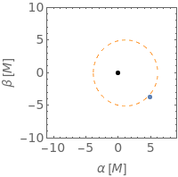
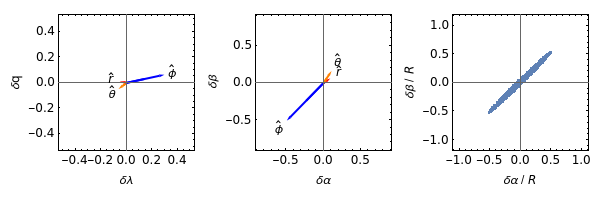
Image shape
If[Not@StringQ@data,shape=Shape[a,data["λ"],Sqrt[data["η"]],rs,θs,ro,data["νrs"],data["νθs"]]]Print", , : the unit base vectors of the spherical coordinate system, normalized to length 1.\nHere they are mapped to the λ-η plane and α-β plane."Print["Stretch rates of principal axes: ",shape[[2]][[1;;2]]]Print["Magnification rate of area: ",shape[[2]][[3]]]
⋀
r
⋀
θ
⋀
ϕ
Out[]=
,{0.740902,0.0412764,0.0305817}
⋀
r
⋀
θ
⋀
ϕ
Stretch rates of principal axes: {0.740902,0.0412764}
Magnification rate of area: 0.0305817
Ex2: Higher-order image in the paper
Ex2: Higher-order image in the paper
Example of a higher-order image: the image in Table II of the original paper.
N=6
In[]:=
a=;rs=10;θs=;θo=;ϕo=π;ro=1000;νrs=-1;νθs=-1;(*Settheguessedvaluesof(rc,lg|d|)andopttofindaimageandextractdetailedinformation.*)rc$seed=2.5;lgAbsd$seed=-6.2;opt="out";(*d>0*)data=FindImage[a,rs,θs,ro,νrs,νθs,θo,ϕo,{rc$seed,lgAbsd$seed},opt,"WorkingPrecision"->80];If[StringQ@data,Print[data],Grid[Transpose@{Keys@data,Values@data},Frame->{All,All}]]
8
10
89.9π
180
17π
180
45
180
Out[]=
a | 0.80000000000000000000000000000000000000000000000000000000000000000000000000000000 |
λ | 0.723713611022987343067150182826630235922206208822571121650780630691568982122953 |
η | 21.06768236776703749022160619941432073193955470149079976122194777156013403694117 |
rs | 10.0000000000000000000000000000000000000000000000000000000000000000000000000000000 |
θs | 1.5690509975429023370452341623604297637939453125000000000000000000000000000000000 |
ro | 1000.00000000000000000000000000000000000000000000000000000000000000000000000000000 |
τo | 4.310427333560645089071103133087662304396868726529033038516678164080586960532734 |
θf | 0.29670597283903602807702743064306416128528822105209332753652254482907154948259 |
ϕf | 25.918139392115794217316807912055898794626647544844623023043292886539485352 |
tf | 1113.20303284468824418812380537277453648552285208115096547859412491858337094 |
θo-θf | 0.× -78 10 |
Sin ϕf-ϕo 2 | 0.× -74 10 |
m | 6 |
nhalf | 6.418964141924416324260807352795705370085466739337583191319099449423850675182867 |
Mod[ϕf, 2π] | 0.785398163397448309615660845819875721049292349843776455243736148076954102 |
α | -2.4753202835045297693164853104200260087326010602200079434984228466773693079438 |
β | -4.0061858763461833445236030641880653658000638338572326776387494089824063972701 |
νrs | -1 |
νθs | -1 |
rc | 2.5033194884120693328264349707419299431853495508530649782197286466307655458456036 |
d | 6.714319053434275479707183790892271334413483810743048670820446996166740513418953× -7 10 |
r1 | -5.404737192772082182821110442698795893650609396292585765267814768777220861874 |
r2 | 0.398097582425267361433615217867980695043761790602359667810566342189303839102 |
r3 | 2.50242117276920099129712379776210934834922763629771033621787344889943888 |
r4 | 2.50421843757761383009037142706870585025761996939251576123937497768847814 |
w0 | 0.98814195001091714781159482498650224056912952917079862380659713302033023140764 |
radial_integrals | {4.310427333560645089071103133087662304396868726529033038516678164080586960532734,6.4906077055226242545332238381861421805889447200762392323293013674554544101,1111.87712712079131936721846007857318098067393955087231874940455887535642340} |
angular_integrals | {4.31042733356064508907110313308766230439686872652903303851667816408058696053273,26.8442259350793010466702771037558168555272791142057741813750536226038007344,2.071727693588945032664602022189617976326425828560385514358696942542105530809} |
3 D demonstration of the geodesic . Increase smax to extend the geodesic .
smax=70;If[Not@StringQ@data,Demo[a,data["λ"],data["η"],νrs,νθs,rs,θs,0,smax]]
End point: {r, θ, ϕ} = {21.72299222185203174,0.4908162395012231617,25.677720142224112821} for s = 70
Out[]=

In[]:=
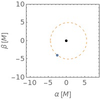
(*Imageplane*)Print["The image plane:\nblack——BH; orange——critical curve; blue——image"]cc$up=ParametricPlot[{αc[rc,a,θo],βc[rc,a,θo]},{rc,rcRange[a][[1]],rcRange[a][[2]]},AspectRatio1,FrameTrue,FrameStyle14,FrameLabel{StringJoin["α [",ToString@TraditionalForm[M],"]"],StringJoin["β [",ToString@TraditionalForm[M],"]"]},LabelStyle14,AxesFalse,PlotStyle->Directive[Dashed,Orange,Thickness[0.005]],PlotPoints100];cc$down=ParametricPlot[{αc[rc,a,θo],-βc[rc,a,θo]},{rc,rcRange[a][[1]],rcRange[a][[2]]},PlotStyle->Directive[Dashed,Orange,Thickness[0.005]],PlotPoints100];plotimage=ListPlot[{{data["α"],data["β"]}},PlotStyleDirective[PointSize[0.03]]];plotBH=ListPlot[{{0,0}},PlotStyleDirective[Black,PointSize[0.03]]];Show[cc$up,cc$down,plotimage,plotBH,PlotRange->{{-10,8},{-9,9}},ImageSize->200]
The image plane:black——BH; orange——critical curve; blue——image
Out[]=
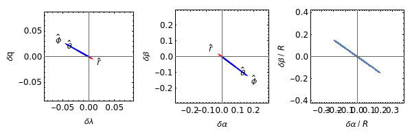
In[]:=
(*Imageshape*)If[Not@StringQ@data,shape=Shape[a,data["λ"],Sqrt[data["η"]],rs,θs,ro,data["νrs"],data["νθs"]]]Print", , : the unit base vectors of the spherical coordinate system, normalized to length 1.\nHere they are mapped to the λ-η plane and α-β plane."Print["Stretch rates of principal axes: ",shape[[2]][[1;;2]]]Print["Magnification rate of area: ",shape[[2]][[3]]]
⋀
r
⋀
θ
⋀
ϕ
Out[]=
,1.44829×}
,{0.238949,6.06108×
-8
10
-8
10
⋀
r
⋀
θ
⋀
ϕ
Stretch rates of principal axes: {0.238949,6.06108×}
-8
10
Magnification rate of area: 1.44829×
-8
10
CITE THIS NOTEBOOK
CITE THIS NOTEBOOK
Forward ray tracing and hot spots in Kerr spacetime
by Lihang Zhou
Wolfram Community, STAFF PICKS, April 16, 2025
https://community.wolfram.com/groups/-/m/t/3444948
by Lihang Zhou
Wolfram Community, STAFF PICKS, April 16, 2025
https://community.wolfram.com/groups/-/m/t/3444948