This study employs an agent-based modeling (ABM) framework, inspired by molecular dynamics, to investigate the mechanisms governing wealth distribution. The methodological scope involves a simulation of 100 agents where economic exchanges are modeled as collisions under different transaction protocols. These protocols include a Fixed Wealth Model and the more complex Affine Wealth Model, which is distinguished by its capacity to accommodate agents with negative wealth (debt). A central objective is to quantify the effects of specific policy interventions on systemic inequality as measured by the Gini index. The investigation systematically examines how parameters representing a universal basic income, a proportional wealth tax, and allowing for agent debt alter wealth stratification.
Introduction
Introduction
Understanding the mechanisms that drive the distribution of wealth is a foundational challenge in economics. While traditional macroeconomic models provide valuable insights, they often rely on high-level abstractions or assumptions of perfect rationality that may not fully capture the stochastic and heterogeneous nature of individual economic decisions. An alternative approach is to use agent-based modeling (ABM), which allows for the exploration of emergent, large-scale phenomena from simple, agent-level interactions.
This study employs an ABM framework inspired by principles from molecular dynamics. We construct a digital laboratory where economic participants are modeled as interacting particles within a closed system. The primary objective is to investigate how different transaction protocols and policy interventions shape the evolution of wealth distribution. By simulating collisions between agents as economic exchanges, we can observe how wealth stratifies over time.
We analyze two primary models: Fixed Income Model and the more complex Affine Wealth Model, which introduces systemic bias and allows for agent debt. The resulting wealth distributions are quantified using the Gini Index and visualized with Lorenz curves, providing a clear measure of systemic inequality. This methodology allows us to test how specific rules governing individual exchanges can lead to vastly different macroeconomic outcomes.
Economic Systems and Transactions
Economic Systems and Transactions
To understand the simulations, it’s essential to define the foundational concepts that form the basis of our model economy.
◼
Agents (Market Participants): The fundamental entities in our model are the agents, representing individual participants in an economy. We simulate a system of 100 agents, each capable of possessing and exchanging wealth.
◼
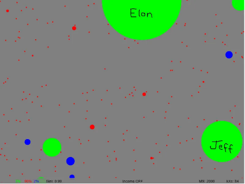
Wealth: This represents the total value of assets held by an agent. In the simulation, it is a numerical value referred to as an agent’s balance. An agent’s wealth is not just a number; it visually determines their size (radius) in the 2D environment, providing an immediate representation of their economic standing.
◼
Transactions: A transaction is a fundamental interaction involving the exchange of wealth between two agents. In our model, a transaction is triggered whenever two agents collide. During a transaction, one agent gives a calculated amount of wealth to the other in exchange for a notional good or service. The rules governing the amount and direction of this wealth transfer are central to the different economic models we explore.
◼
Gini Index: To measure the level of wealth inequality in the system, we use the Gini Index. It is a standard statistical measure that ranges from 0 to 1, where 0 represents perfect equality (all agents have the same wealth) and 1 represents perfect inequality (one agent holds all the wealth). We track the Gini Index over time to observe how the wealth distribution evolves under different economic rules.
computeGini[bals_]:=Module[{n=Length[bals],sorted,total},total=Total[bals];If[n<2||total==0,Return[0]];sorted=Sort[bals];(2*Total[Range[n]*sorted])/(n*total)-(n+1)/n];
◼
Lorenz Curve: As a visual companion to the Gini Index, the Lorenz Curve provides a graphical representation of wealth distribution. It plots the cumulative percentage of the population (from poorest to richest) on the horizontal axis against the cumulative percentage of total wealth they hold on the vertical axis. A perfectly straight diagonal line represents perfect equality, while a curve that bows further away from the diagonal indicates greater inequality.
◼
Economic Policies (Model Parameters): Our digital laboratory allows us to introduce system-wide economic policies by adjusting key parameters. We explore how the following factors influence the Gini Index and overall wealth inequality:
◼
Income: A universal basic income can be introduced, giving each agent a small, fixed amount of wealth at each time step.
◼
Tax: A proportional wealth tax can be applied, removing a small percentage of each agent’s wealth, which can then be redistributed.
◼
Debt: The Affine Wealth Model introduces a more complex system where agents can transact more than their current wealth, effectively allowing them to go into debt.
By manipulating these foundational elements, we can simulate and analyze a variety of economic scenarios.
Modeling Transactions with Hard Spheres
Modeling Transactions with Hard Spheres
To simulate economic activity, we adopt a framework from physics known as a hard-sphere model. In a physical context, this model describes a system of particles (like a gas) where each particle is a perfectly round, hard sphere that interacts with others only when they physically collide. This provides a simplified yet powerful basis for modeling our economy.
The core of our methodology lies in the direct analogy we draw between this physical system and an economic one:
◼
Particles as People: Each hard sphere in the simulation represents an individual economic agent.
◼
Collisions as Transactions: A collision between two spheres is treated as an economic transaction. As long as two agents’ disks overlap, they are in a state of interaction, and a transfer of wealth occurs.
◼
Wealth as Influence: An agent’s wealth is represented by the size of their sphere. This provides a direct visual cue to their economic standing and influences their interaction with others in the shared space.
The value of this model is its ability to abstract the immense complexity of a real-world economy into a system of simple, observable interactions. This allows us to investigate whether complex macroeconomic patterns, such as the persistent tendency for wealth to concentrate, can emerge from simple, unbiased rules at the individual level. This approach is inspired by simulations like those explored by Philip Rosedale [1], which demonstrate that even with fair and random exchanges, a system can naturally drift toward inequality. The core mechanism is that for an agent with less wealth, a transaction that results in a net loss has a much greater relative impact than for a wealthier agent, increasing their risk of economic ruin over time. Our model captures this dynamic by having one agent give a transaction amount to the other in exchange for a notional good or service upon each collision.
Description of the Model
Description of the Model
This study utilizes an agent-based model (ABM) to simulate the evolution of wealth distribution within a population. The model is built on a shared foundation of agents interacting within a 2D environment, with different economic rules applied to govern their transactions. The following sections describe the fundamental design and the specific economic models implemented.
Simulation Design
Simulation Design
Both models share the same fundamental environment and agent properties.
◼
Entities and Environment: The simulation contains 100 agents in a 2D space with periodic boundaries. Each agent has a position, velocity, and a balance (wealth). Their size is represented by a disk whose radius is proportional to their share of the total system wealth.
◼
Interaction: The primary interaction mechanic is a collision. When two agents’ disks overlap, a transaction between them is triggered.
◼
System-Wide Wealth Dynamics: Both models can operate as open systems. A key parameter, enableIncome, controls a universal wealth redistribution mechanism.
◼
Basic Income: When enabled, each agent receives a small, fixed amount of wealth [basicIncome] in every time step.
◼
Wealth Tax (Decay Rate): A decayRate is applied to every agent’s balance in each time step. A rate of less than 1.0 (e.g., 0.99) acts as a proportional wealth tax, removing a small percentage of wealth from the system. A rate of 1.0 means no wealth is removed this way.
Economic Transaction Models
Economic Transaction Models
The core difference between the simulations lies in the rules governing what happens during a transaction.
Fixed Income Model
Fixed Income Model
This model uses a transaction rule with a predefined risk limit and a fair, unbiased outcome, operating within an economy that features wealth redistribution.
◼
Transaction Amount: The amount of wealth at stake is a random fraction of the poorer agent’s balance, further limited by the fractionToRisk parameter. The formula is: Amount = Poorer Balance * RandomReal[{0, fractionToRisk}].
◼
Wealth Transfer: The transfer of wealth is determined by a fair 50/50 coin flip, which randomly decides the direction of the exchange. This means one agent gives the transaction amount to the other in exchange for a notional good or service, with both participants having an equal chance of being the payer or the recipient.
Affine Wealth Model
Affine Wealth Model
This model introduces two key modifications to the classic Yard-Sale model: a credit/debt system and a systemic wealth bias. This creates a more complex economy where agents can transact more than their current wealth.
◼
Transaction Amount: The amount at stake is not limited by the poorer agent’s balance. Instead, it’s a random fraction of the agent’s balance plus a credit/debt buffer, Δ. This allows agents to go into debt. Here, balP represents the poorer agent’s balance, and Min[shiftedBalR, shiftedBalP] resolves to balP + Δ.
shiftedBalR=balR+Δ;shiftedBalP=balP+Δ;amount=RandomReal[{0,Min[shiftedBalR,shiftedBalP]}];
◼
Biased Wealth Transfer: The outcome is determined by a biased coin flip. The probability that wealth flows from the poorer agent to the richer one is controlled by the zeta (ζ) parameter. The probability is calculated as:When ζ > 0, the model creates a “rich-get-richer” feedback loop. When ζ < 0, it creates an egalitarian or “pro-poor” bias. If ζ = 0, this model becomes a pure Yard-Sale model with a fair 50/50 outcome.
P(RicherWins)+0.5
ζ (WealthRicher-WealthPoorer)
AverageWealth
Simulation Setups
Simulation Setups
All simulations are built upon a shared set of foundational parameters that define the environment and the initial state of the economy . To test various economic hypotheses, we then run the simulation under four distinct scenarios, each with different rules governing transactions and wealth dynamics .
Experimental Parameters
Experimental Parameters
The common experimental parameters ensure a consistent starting point for each simulation run .
Fixed Income Model
Fixed Income Model
Module{num=100,balanceInitial=50.0,fractionToRisk=0.1,basicIncome=0.05,decayRate=1.0,enableIncome=False,vMax=1.0,minRadius=0.002,dt=1/100,maxTransactions=250000,positions,velocities,balances,radii,transactions=0,frame=0,giniHistory={},lorenzData={},computeGini,runStep,getColor,giniIndex,averageBalance,moneySupply,finalBalances},
◼
num: This sets the number of agents or individuals in your simulation to 100.
◼
balanceInitial: Each of the 100 agents starts with an initial balance of 50.0 units of currency.
◼
fractionToRisk: In each transaction, agents will risk 10% of their current balance.
◼
basicIncome: This is the amount of basic income that can be added to each agent’s balance in each time step if enableIncome is active.
◼
decayRate: This represents a wealth decay factor. A rate of 1.0 means there is currently no decay. This is similar to a taxation proportional to wealth.
◼
maxTransactions: This is the maximum number of transactions that will occur before the simulation ends.
◼
enableIncome: This will activate the basicIncome of 0.05 for every agent at each time step, injecting new money into the economy.
Affine Wealth Model
Affine Wealth Model
Module{num=100,balanceInitial=50.0,basicIncome=0.05,decayRate=0.99,enableIncome=False,vMin=0.1,vMax=1,minRadius=0.002,dt=1/100,maxTransactions=10000,zeta=0.0,κ=0.08,Δ,frame=0,transactions=0,giniIndex=0,averageBalance,moneySupply,giniHistory={},finalBalances={},lorenzData={},pos,vel,balance,radius,nf},
◼
num: This sets the number of agents or individuals in your simulation to 100.
◼
balanceInitial: Each of the 100 agents starts with an initial balance of 50.0 units of currency.
◼
basicIncome: This is the amount of basic income that can be added to each agent’s balance in each time step if enableIncome is active.
◼
decayRate: This factor introduces a wealth decay of 1% (1.0 - 0.99) on each agent’s balance at every time step. This represents a form of wealth tax or redistribution.
◼
maxTransactions: This is the maximum number of transactions that will occur before the simulation ends.
◼
zeta: Represents the Wealth Attained Advantage (WAA) parameter, a systematic bias favoring the wealthier agent in a transaction to drive wealth concentration.
◼
kappa(κ): Acts as the wealth distribution shift parameter, allowing the model to incorporate negative balances (debt) for greater realism.
Results
Results
Fixed Wealth Model
Fixed Wealth Model
Rapid Evolution to Inequality
Rapid Evolution to Inequality
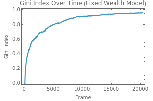
The simulation begins from a state of perfect equality (Gini coefficient = 0). The system’s evolution is governed by purely multiplicative random transactions, where the amount exchanged is a fraction of an agent’s wealth. The Gini coefficient exhibits a phase of rapid, near-exponential growth, eventually approaching a steady-state equilibrium near 0.96. This trajectory is a classic indicator of wealth condensation, a phenomenon where stochastic exchanges in a closed system lead to a near-monopolistic outcome, with one agent accumulating almost all the wealth.
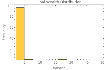
Characterization of the Final Wealth Distribution
Characterization of the Final Wealth Distribution
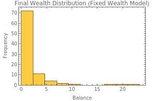
The final wealth distribution, as depicted in the histogram, confirms the outcome predicted by the Gini trajectory. The distribution is extremely skewed, forming an L-shaped or reverse-J-shaped curve characteristic of high inequality. The vast majority of the probability mass is concentrated at the lowest end of the wealth spectrum, with over 70% of the agent population possessing near-zero balances. The distribution’s long, sparse tail signifies that a very small number of agents hold a disproportionately large fraction of the total wealth.
Code
Code
Fixed Wealth Model with Income
Fixed Wealth Model with Income
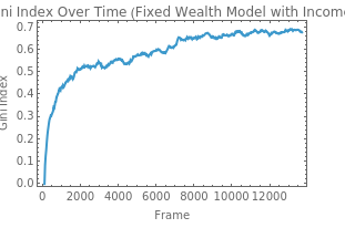
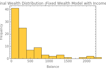
This simulation introduces a universal basic income, where every agent receives a small, constant amount of wealth at each time step. While significant inequality still emerges, the results differ markedly from the baseline model without income.
Quantitative Impact on the Gini Coefficient
Quantitative Impact on the Gini Coefficient
The introduction of an additive income term fundamentally alters the system’s trajectory toward inequality. The Gini coefficient, which measures the statistical dispersion of wealth, stabilizes in the approximate range of 0.6 to 0.7. This is a substantial reduction from the Gini coefficient of the baseline model, which approached a near-total inequality of approximately 0.96.
The term “basicIncome” counteracts the wealth-condensing effect inherent in the purely multiplicative transaction process. In the baseline model, that process leads to a state of near-monopoly. The additive income ensures a persistent, system-wide wealth injection, preventing the terminal decay of any agent’s wealth and thereby lowering the ceiling of achievable inequality.
The term “basicIncome” counteracts the wealth-condensing effect inherent in the purely multiplicative transaction process. In the baseline model, that process leads to a state of near-monopoly. The additive income ensures a persistent, system-wide wealth injection, preventing the terminal decay of any agent’s wealth and thereby lowering the ceiling of achievable inequality.
Modification of the Final Wealth Distribution
Modification of the Final Wealth Distribution
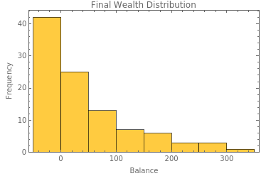
The final wealth distribution transitions from the extreme L-shape seen in the baseline model to a less skewed, long-tailed distribution, characteristic of a log-normal or Gamma distribution.
While still skewed, the distribution’s modal class is situated at a non-zero wealth level, containing approximately 40 agents. Crucially, a significant portion of the probability mass is distributed across intermediate wealth values, forming a visible “body” in the histogram that was absent in the baseline.
While still skewed, the distribution’s modal class is situated at a non-zero wealth level, containing approximately 40 agents. Crucially, a significant portion of the probability mass is distributed across intermediate wealth values, forming a visible “body” in the histogram that was absent in the baseline.
Code
Code
Fixed Wealth Model with Income & Tax
Fixed Wealth Model with Income & Tax
Analysis of the Fixed Wealth Model with Additive Income and Proportional Wealth Tax
Analysis of the Fixed Wealth Model with Additive Income and Proportional Wealth Tax
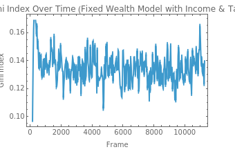
This simulation introduces a decayRate of 0.99, which functions as a 1% proportional wealth tax, alongside the additive basic income. The interplay between the inequality-driving random exchanges and these two powerful redistributive forces results in a dramatically different and highly equitable system.
Suppression of Inequality and Gini Coefficient Stabilization
Suppression of Inequality and Gini Coefficient Stabilization
The Gini coefficient is suppressed to a very low value, fluctuating within a narrow band of approximately 0.10 to 0.16, which indicates a state of high and stable equality. The additive income provides a constant uplifting force for agents with lower balances, while the proportional tax acts as a strong, mean-reverting force by disproportionately reducing the wealth of the richest agents. This combination of mechanisms effectively neutralizes the wealth-condensing tendency of the random exchanges.
Resulting Wealth Distribution
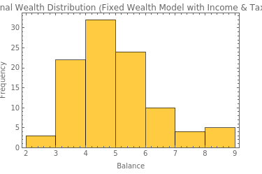
Resulting Wealth Distribution
The final wealth distribution is transformed from the heavily skewed curves of the previous models into a symmetric, unimodal distribution that closely resembles a Gaussian curve. The majority of the population is clustered around a central mean value, and the rapidly decaying tails of the histogram indicate a near-absence of extreme outliers. This statistical signature is a direct result of the strong redistributive pressures that curtail large deviations from the average wealth.
Code
Code
Affine Wealth Model (zeta = 0)
Affine Wealth Model (zeta = 0)
Affine Wealth Model with Debt and Condensation
Affine Wealth Model with Debt and Condensation
The simulation demonstrates a key capability of the Affine Wealth Model (AWM): its ability to account for agents with negative wealth (debt). This feature leads to unique and extreme characteristics in the measures of inequality.
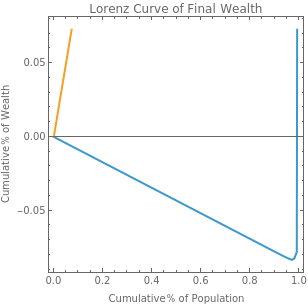
Lorenz Curve with Negative Wealth
Lorenz Curve with Negative Wealth
The Lorenz curve generated by the simulation deviates from the standard form by entering the fourth quadrant from the origin. This behavior is a key feature of the Affine Wealth Model (AWM), which is specifically formulated to allow for agents with negative net worth (debt). The model achieves this by incorporating a wealth shift parameter, κ, which enables transactions that can result in an agent’s balance becoming negative.
Gini Coefficient in a System with Debt
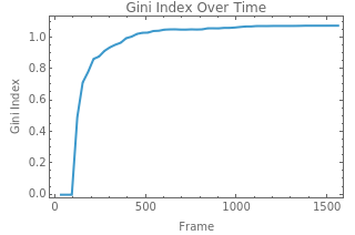
Gini Coefficient in a System with Debt
The Gini coefficient evolves to a steady-state value exceeding 1.0. A Gini coefficient greater than unity is a known, though extreme, outcome in systems with a significant number of negative-wealth agents.
The Gini coefficient quantifies the area between the Lorenz curve and the line of perfect equality. When the Lorenz curve extends below the horizontal axis, the total area of deviation can exceed the reference area under the diagonal, resulting in a value greater than 1. This signifies a state of wealth polarization more extreme than a simple monopoly (where G = 1). It describes a system characterized by both the condensation of wealth into a single entity and the simultaneous indebtedness of the rest of the population. This interpretation is corroborated by the final wealth distribution, which shows nearly the entire agent population with negative balances, and by the system visualization.
The Gini coefficient quantifies the area between the Lorenz curve and the line of perfect equality. When the Lorenz curve extends below the horizontal axis, the total area of deviation can exceed the reference area under the diagonal, resulting in a value greater than 1. This signifies a state of wealth polarization more extreme than a simple monopoly (where G = 1). It describes a system characterized by both the condensation of wealth into a single entity and the simultaneous indebtedness of the rest of the population. This interpretation is corroborated by the final wealth distribution, which shows nearly the entire agent population with negative balances, and by the system visualization.
Code
Code
Affine Wealth Model (zeta = -0.2)
Affine Wealth Model (zeta = -0.2)
Affine Wealth Model with an Egalitarian Bias
Affine Wealth Model with an Egalitarian Bias
This simulation implements the Affine Wealth Model (AWM) with a negative Wealth Attained Advantage (WAA) parameter (zeta = -0.2). This configuration introduces a systematic bias that favors the poorer agent in every transaction, creating a continuous, “pro-poor” or egalitarian pressure within the system.
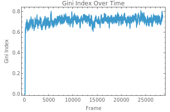
Gini Coefficient Equilibrium
Gini Coefficient Equilibrium
The Gini coefficient rapidly rises from an initial state of equality (Gini = 0) and then stabilizes, fluctuating in a dynamic equilibrium around 0.7 to 0.75. This outcome is the result of two competing dynamics:
◼
The inherent multiplicative randomness of the asset-exchange model, which drives the system toward inequality.
◼
The egalitarian bias from the negative zeta, which acts as a powerful mean-reverting force by continuously transferring a fraction of wealth from richer to poorer agents.
The resulting Gini coefficient represents the equilibrium point where these two opposing forces are balanced. The bias prevents the extreme wealth condensation seen in the baseline model (where Gini approaches 1), but it does not completely eliminate inequality.
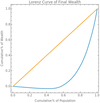
Final Wealth Distribution
Final Wealth Distribution
The final distribution of wealth is a skewed, long-tailed curve, which is characteristic of a system with significant inequality. A large fraction of the population possesses low levels of wealth, while a progressively smaller number of agents hold higher balances. Although the model permits debt (via the kappa parameter), the strong “pro-poor” pressure from zeta is sufficient to prevent widespread negative balances, as confirmed by the Lorenz Curve, which remains entirely within the first quadrant.
Code
Code
Limitations
Limitations
◼
No Wealth Creation: The model simulates only the exchange of existing wealth, not its creation through production, innovation, or entrepreneurship.
◼
Baseline for Agent Behavior : The model intentionally uses agents with simple, fixed rules to create a controlled environment . This provides a baseline understanding of core interactions, paving the way for future versions to incorporate more complex human behaviors and strategic decision - making .
◼
Simple System for Ease of Simulation: The model cannot replicate essential economic systems like formal labor markets, credit systems (banks, interest rates), and does not account for inflation.
◼
Dynamics in a Stable Population: Agents are immortal, meaning the model cannot represent the economic effects of aging, retirement, or the transfer of wealth between generations. This can be accounted for in future work.
Concluding Remarks
Concluding Remarks
The effectiveness of an agent-based paradigm, similar to molecular dynamics, for examining the emergent characteristics of economic systems is demonstrated in this paper. The model effectively replicated a variety of wealth distributions, from severe wealth condensation to a stable, egalitarian equilibrium, by modeling transactions as collisions between agents. These distributions resulted directly from the repetitive application of straightforward, agent-level rules.
The main advantage of this strategy is its adaptability. Different economic models, such as the more intricate Affine Wealth and Fixed Wealth models, might be directly implemented and compared thanks to the framework. This flexibility was essential for methodically examining the effects of many factors, including proportional wealth decay, additive income, and systemic transaction biases.
The effectiveness of this approach offers a strong starting point for further study. Future research will compare the consequences of open and closed economic systems and try sophisticated strategies like wealth redistribution and an adaptive tax aimed at a stable Gini Index. In the end, our study confirms that agent-based modeling is a very flexible and perceptive approach to investigating the connection between macro-level distributional results and micro-level economic norms.
Keywords
Keywords
◼
WSS25
◼
Agent-Based Modeling
◼
Finance
◼
Wealth Distribution
Acknowledgments
Acknowledgments
First and foremost, I would like to thank Stephanie for the incredible opportunity to participate in the Wolfram Summer School 2025. When faced with visa complications, her support in enabling my virtual attendance was truly invaluable.
I cannot overstate my gratitude for my mentor, Sotiris Michos. His patient guidance and clear explanations were a constant source of support, and he skillfully ensured that my work was as enjoyable as it was challenging.
My thanks are also due to James Wiles for his insightful feedback that sharpened the focus of my project; I hope it is a line of inquiry I can pursue further. And to Stephen Wolfram, I am deeply grateful for perceiving my interests so keenly and assigning me the most fascinating project I could have imagined, as well as for the generous resources he provided.
References
References
1
.Rosedale, P. (2021, January 27). Why do the rich get richer? Substack. https://philiprosedale.substack.com/p/why-do-the-rich-get-richer
2
.Li, J., Boghosian, B. M., & Li, C. (2016, January). The Affine Wealth Model: An agent-based model of asset exchange that allows for negative-wealth agents and its empirical validation. arXiv. https://doi.org/10.48550/arxiv.1604.02370
Cite This Notebook
Cite This Notebook
Wealth exchange in agent-based systems
by Arul Singh
Wolfram Community, July 9, 2025
https://community.wolfram.com/groups/-/m/t/3497933
by Arul Singh
Wolfram Community, July 9, 2025
https://community.wolfram.com/groups/-/m/t/3497933